symjax.tensor

Implements the NumPy API, using the primitives in jax.lax. As SymJAX follows the JAX restrictions, not all NumPy functins are present.

• Notably, since JAX arrays are immutable, NumPy APIs that mutate arrays in-place cannot be implemented in JAX. However, often JAX is able to provide a alternative API that is purely functional. For example, instead of in-place array updates (x[i] = y), JAX provides an alternative pure indexed update function jax.ops.index_update().
• NumPy is very aggressive at promoting values to float64 type. JAX sometimes is less aggressive about type promotion.

Finally, since SymJAX uses jit-compilation, any function that returns data-dependent output shapes are incompatible and thus not implemented. In fact, The XLA compiler requires that shapes of arrays be known at compile time. While it would be possible to provide. Thus an implementation of an API such as numpy.nonzero(), we would be unable to JIT-compile it because the shape of its output depends on the contents of the input data.

Not every function in NumPy is implemented; contributions are welcome!

Numpy Ops

abs(x)	Calculate the absolute value element-wise.
absolute(x)	Calculate the absolute value element-wise.
add(x1, x2)	Add arguments element-wise.
all(a[, axis, out, keepdims])	Test whether all array elements along a given axis evaluate to True.
allclose(a, b[, rtol, atol, equal_nan])	Returns True if two arrays are element-wise equal within a tolerance.
alltrue(a[, axis, out, keepdims])	Test whether all array elements along a given axis evaluate to True.
amax(a[, axis, out, keepdims, initial, where])	Return the maximum of an array or maximum along an axis.
amin(a[, axis, out, keepdims, initial, where])	Return the minimum of an array or minimum along an axis.
angle(z)	Return the angle of the complex argument.
any(a[, axis, out, keepdims])	Test whether any array element along a given axis evaluates to True.
append(arr, values[, axis])	Append values to the end of an array.
arange(start[, stop, step, dtype])	Return evenly spaced values within a given interval.
arccos(x)	Trigonometric inverse cosine, element-wise.
arccosh(x)	Inverse hyperbolic cosine, element-wise.
arcsin(x)	Inverse sine, element-wise.
arcsinh(x)	Inverse hyperbolic sine element-wise.
arctan(x)	Trigonometric inverse tangent, element-wise.
arctan2(x1, x2)	Element-wise arc tangent of x1/x2 choosing the quadrant correctly.
arctanh(x)	Inverse hyperbolic tangent element-wise.
argmax(a[, axis, out])	Returns the indices of the maximum values along an axis.
argmin(a[, axis, out])	Returns the indices of the minimum values along an axis.
argsort(a[, axis, kind, order])	Returns the indices that would sort an array.
argwhere(a)	Find the indices of array elements that are non-zero, grouped by element.
around(a[, decimals, out])	Round an array to the given number of decimals.
array(object[, dtype, copy, order, ndmin])	Create an array.
array_repr
array_str
asarray(a[, dtype, order])	Convert the input to an array.
atleast_1d(*arys)	Convert inputs to arrays with at least one dimension.
atleast_2d(*arys)	View inputs as arrays with at least two dimensions.
atleast_3d(*arys)	View inputs as arrays with at least three dimensions.
bartlett
bincount(x[, weights, minlength, length])	Count number of occurrences of each value in array of non-negative ints.
bitwise_and(x1, x2)	Compute the bit-wise AND of two arrays element-wise.
bitwise_not(x)	Compute bit-wise inversion, or bit-wise NOT, element-wise.
bitwise_or(x1, x2)	Compute the bit-wise OR of two arrays element-wise.
bitwise_xor(x1, x2)	Compute the bit-wise XOR of two arrays element-wise.
blackman
block(arrays)	Assemble an nd-array from nested lists of blocks.
broadcast_arrays(*args)	Like Numpy’s broadcast_arrays but doesn’t return views.
broadcast_to(arr, shape)	Broadcast an array to a new shape.
can_cast(from_, to[, casting])	Returns True if cast between data types can occur according to the casting rule.
ceil(x)	Return the ceiling of the input, element-wise.
clip(a[, a_min, a_max, out])	Clip (limit) the values in an array.
column_stack(tup)	Stack 1-D arrays as columns into a 2-D array.
compress(condition, a[, axis, out])	Return selected slices of an array along given axis.
concatenate(arrays[, axis])	Join a sequence of arrays along an existing axis.
conj(x)	Return the complex conjugate, element-wise.
conjugate(x)	Return the complex conjugate, element-wise.
convolve(a, v[, mode, precision])	Returns the discrete, linear convolution of two one-dimensional sequences.
copysign(x1, x2)	Change the sign of x1 to that of x2, element-wise.
corrcoef(x[, y, rowvar])	Return Pearson product-moment correlation coefficients.
correlate(a, v[, mode, precision])	Cross-correlation of two 1-dimensional sequences.
cos(x)	Cosine element-wise.
cosh(x)	Hyperbolic cosine, element-wise.
count_nonzero(a[, axis, keepdims])	Counts the number of non-zero values in the array a.
cov(m[, y, rowvar, bias, ddof, fweights, …])	Estimate a covariance matrix, given data and weights.
cross(a, b[, axisa, axisb, axisc, axis])	Return the cross product of two (arrays of) vectors.
cumsum(a[, axis, dtype, out])	Return the cumulative sum of the elements along a given axis.
cumprod(a[, axis, dtype, out])	Return the cumulative product of elements along a given axis.
cumproduct(a[, axis, dtype, out])	Return the cumulative product of elements along a given axis.
deg2rad(x)	Convert angles from degrees to radians.
degrees(x)	Convert angles from radians to degrees.
diag(v[, k])	Extract a diagonal or construct a diagonal array.
diag_indices(n[, ndim])	Return the indices to access the main diagonal of an array.
diag_indices_from(arr)	Return the indices to access the main diagonal of an n-dimensional array.
diagflat(v[, k])	Create a two-dimensional array with the flattened input as a diagonal.
diagonal(a[, offset, axis1, axis2])	Return specified diagonals.
digitize
divide(x1, x2)	Returns a true division of the inputs, element-wise.
divmod(x1, x2)	Return element-wise quotient and remainder simultaneously.
dot(a, b, *[, precision])	Dot product of two arrays.
dsplit(ary, indices_or_sections)	Split array into multiple sub-arrays along the 3rd axis (depth).
dstack(tup)	Stack arrays in sequence depth wise (along third axis).
ediff1d(ary[, to_end, to_begin])	The differences between consecutive elements of an array.
einsum(*operands[, out, optimize, precision])	Evaluates the Einstein summation convention on the operands.
equal(x1, x2)	Return (x1 == x2) element-wise.
empty(shape[, dtype])	Return a new array of given shape and type, filled with zeros.
empty_like(a[, dtype, shape])	Return an array of zeros with the same shape and type as a given array.
exp(x)	Calculate the exponential of all elements in the input array.
exp2(x)	Calculate 2**p for all p in the input array.
expand_dims(a, axis, Tuple[int, …]])	Expand the shape of an array.
expm1(x)	Calculate exp(x) - 1 for all elements in the array.
extract(condition, arr)	Return the elements of an array that satisfy some condition.
eye(N[, M, k, dtype])	Return a 2-D array with ones on the diagonal and zeros elsewhere.
fabs(x)	Compute the absolute values element-wise.
fix(x[, out])	Round to nearest integer towards zero.
flatnonzero(a)	Return indices that are non-zero in the flattened version of a.
flip(m[, axis])	Reverse the order of elements in an array along the given axis.
fliplr(m)	Flip array in the left/right direction.
flipud(m)	Flip array in the up/down direction.
float_power(x1, x2)	First array elements raised to powers from second array, element-wise.
floor(x)	Return the floor of the input, element-wise.
floor_divide(x1, x2)	Return the largest integer smaller or equal to the division of the inputs.
fmax(x1, x2)	Element-wise maximum of array elements.
fmin(x1, x2)	Element-wise minimum of array elements.
fmod(x1, x2)	Return the element-wise remainder of division.
frexp
full(shape, fill_value[, dtype])	Return a new array of given shape and type, filled with fill_value.
full_like(a, fill_value[, dtype, shape])	Return a full array with the same shape and type as a given array.
gcd(x1, x2)	Returns the greatest common divisor of |x1| and |x2|
geomspace(start, stop[, num, endpoint, …])	Return numbers spaced evenly on a log scale (a geometric progression).
greater(x1, x2)	Return the truth value of (x1 > x2) element-wise.
greater_equal(x1, x2)	Return the truth value of (x1 >= x2) element-wise.
hamming
hanning
heaviside(x1, x2)	Compute the Heaviside step function.
histogram(a[, bins, range, weights, density])	Compute the histogram of a set of data.
histogram_bin_edges(a[, bins, range, weights])	Function to calculate only the edges of the bins used by the histogram
hsplit(ary, indices_or_sections)	Split an array into multiple sub-arrays horizontally (column-wise).
hstack(tup)	Stack arrays in sequence horizontally (column wise).
hypot(x1, x2)	Given the “legs” of a right triangle, return its hypotenuse.
identity(n[, dtype])	Return the identity array.
imag(val)	Return the imaginary part of the complex argument.
in1d(ar1, ar2[, assume_unique, invert])	Test whether each element of a 1-D array is also present in a second array.
indices(dimensions[, dtype, sparse])	Return an array representing the indices of a grid.
inner(a, b, *[, precision])	Inner product of two arrays.
isclose(a, b[, rtol, atol, equal_nan])	Returns a boolean array where two arrays are element-wise equal within a
iscomplex(x)	Returns a bool array, where True if input element is complex.
isfinite(x)	Test element-wise for finiteness (not infinity or not Not a Number).
isin(element, test_elements[, …])	Calculates element in test_elements, broadcasting over element only.
isinf(x)	Test element-wise for positive or negative infinity.
isnan(x)	Test element-wise for NaN and return result as a boolean array.
isneginf(x[, out])	Test element-wise for negative infinity, return result as bool array.
isposinf(x[, out])	Test element-wise for positive infinity, return result as bool array.
isreal(x)	Returns a bool array, where True if input element is real.
isscalar(element)	Returns True if the type of element is a scalar type.
issubdtype(arg1, arg2)	Returns True if first argument is a typecode lower/equal in type hierarchy.
issubsctype(arg1, arg2)	Determine if the first argument is a subclass of the second argument.
ix_(*args)	Construct an open mesh from multiple sequences.
kaiser
kron(a, b)	Kronecker product of two arrays.
lcm(x1, x2)	Returns the lowest common multiple of |x1| and |x2|
ldexp(x1, x2)	Returns x1 * 2**x2, element-wise.
left_shift(x1, x2)	Shift the bits of an integer to the left.
less(x1, x2)	Return the truth value of (x1 < x2) element-wise.
less_equal(x1, x2)	Return the truth value of (x1 =< x2) element-wise.
linspace(start, stop[, num, endpoint, …])	Return evenly spaced numbers over a specified interval.
log(x)	Natural logarithm, element-wise.
log10(x)	Return the base 10 logarithm of the input array, element-wise.
log1p(x)	Return the natural logarithm of one plus the input array, element-wise.
log2(x)	Base-2 logarithm of x.
logaddexp(x1, x2)	Logarithm of the sum of exponentiations of the inputs.
logaddexp2(x1, x2)	Logarithm of the sum of exponentiations of the inputs in base-2.
logical_and(*args)	Compute the truth value of x1 AND x2 element-wise.
logical_not(*args)	Compute the truth value of NOT x element-wise.
logical_or(*args)	Compute the truth value of x1 OR x2 element-wise.
logical_xor(*args)	Compute the truth value of x1 XOR x2, element-wise.
logspace(start, stop[, num, endpoint, base, …])	Return numbers spaced evenly on a log scale.
matmul(a, b, *[, precision])	Matrix product of two arrays.
max(a[, axis, out, keepdims, initial, where])	Return the maximum of an array or maximum along an axis.
maximum(x1, x2)	Element-wise maximum of array elements.
mean(a[, axis, dtype, out, keepdims])	Compute the arithmetic mean along the specified axis.
median(a[, axis, out, overwrite_input, keepdims])	Compute the median along the specified axis.
meshgrid(*args, **kwargs)	Return coordinate matrices from coordinate vectors.
min(a[, axis, out, keepdims, initial, where])	Return the minimum of an array or minimum along an axis.
minimum(x1, x2)	Element-wise minimum of array elements.
mod(x1, x2)	Return element-wise remainder of division.
moveaxis(a, source, destination)	Move axes of an array to new positions.
msort(a)	Return a copy of an array sorted along the first axis.
multiply(x1, x2)	Multiply arguments element-wise.
nan_to_num(x[, copy, nan, posinf, neginf])	Replace NaN with zero and infinity with large finite numbers (default
nanargmax(a[, axis])	Return the indices of the maximum values in the specified axis ignoring
nanargmin(a[, axis])	Return the indices of the minimum values in the specified axis ignoring
nancumprod(a[, axis, dtype, out])	Return the cumulative product of array elements over a given axis treating Not a
nancumsum(a[, axis, dtype, out])	Return the cumulative sum of array elements over a given axis treating Not a
nanmax(a[, axis, out, keepdims])	Return the maximum of an array or maximum along an axis, ignoring any
nanmedian(a[, axis, out, overwrite_input, …])	Compute the median along the specified axis, while ignoring NaNs.
nanmin(a[, axis, out, keepdims])	Return minimum of an array or minimum along an axis, ignoring any NaNs.
nanpercentile(a, q[, axis, out, …])	Compute the qth percentile of the data along the specified axis,
nanprod(a[, axis, dtype, out, keepdims])	Return the product of array elements over a given axis treating Not a
nanquantile(a, q[, axis, out, …])	Compute the qth quantile of the data along the specified axis,
nansum(a[, axis, dtype, out, keepdims])	Return the sum of array elements over a given axis treating Not a
negative(x)	Numerical negative, element-wise.
nextafter(x1, x2)	Return the next floating-point value after x1 towards x2, element-wise.
nonzero(a)	Return the indices of the elements that are non-zero.
not_equal(x1, x2)	Return (x1 != x2) element-wise.
ones(shape[, dtype])	Return a new array of given shape and type, filled with ones.
ones_like(input[, detach])
outer(a, b[, out])	Compute the outer product of two vectors.
packbits
pad(array, pad_width[, mode, …])	Pad an array.
percentile(a, q[, axis, out, …])	Compute the q-th percentile of the data along the specified axis.
polyadd(a1, a2)	Find the sum of two polynomials.
polyder(p[, m])	Return the derivative of the specified order of a polynomial.
polymul(a1, a2, *[, trim_leading_zeros])	Find the product of two polynomials.
polysub(a1, a2)	Difference (subtraction) of two polynomials.
polyval(p, x)	Evaluate a polynomial at specific values.
power(x1, x2)	First array elements raised to powers from second array, element-wise.
positive(x)	Numerical positive, element-wise.
prod(a[, axis, dtype, out, keepdims, …])	Return the product of array elements over a given axis.
product(a[, axis, dtype, out, keepdims, …])	Return the product of array elements over a given axis.
promote_types(a, b)	Returns the type to which a binary operation should cast its arguments.
ptp(a[, axis, out, keepdims])	Range of values (maximum - minimum) along an axis.
quantile(a, q[, axis, out, overwrite_input, …])	Compute the q-th quantile of the data along the specified axis.
rad2deg(x)	Convert angles from radians to degrees.
radians(x)	Convert angles from degrees to radians.
ravel(a[, order])	Return a contiguous flattened array.
real(val)	Return the real part of the complex argument.
reciprocal(x)	Return the reciprocal of the argument, element-wise.
remainder(x1, x2)	Return element-wise remainder of division.
repeat(a, repeats[, axis, total_repeat_length])	Repeat elements of an array.
reshape(a, newshape[, order])	Gives a new shape to an array without changing its data.
result_type(*args)	Returns the type that results from applying the NumPy
right_shift(x1, x2)	Shift the bits of an integer to the right.
rint(x)	Round elements of the array to the nearest integer.
roll(a, shift[, axis])	Roll array elements along a given axis.
rollaxis(a, axis[, start])	Roll the specified axis backwards, until it lies in a given position.
roots(p, *[, strip_zeros])	Return the roots of a polynomial with coefficients given in p.
rot90(m[, k, axes])	Rotate an array by 90 degrees in the plane specified by axes.
round(a[, decimals, out])	Round an array to the given number of decimals.
row_stack(tup)	Stack arrays in sequence vertically (row wise).
searchsorted
select(condlist, choicelist[, default])	Return an array drawn from elements in choicelist, depending on conditions.
sign(x)	Returns an element-wise indication of the sign of a number.
signbit(x)	Returns element-wise True where signbit is set (less than zero).
sin(x)	Trigonometric sine, element-wise.
sinc(x)	Return the sinc function.
sinh(x)	Hyperbolic sine, element-wise.
sometrue(a[, axis, out, keepdims])	Test whether any array element along a given axis evaluates to True.
sort(a[, axis, kind, order])	Return a sorted copy of an array.
split(ary, indices_or_sections[, axis])	Split an array into multiple sub-arrays as views into ary.
sqrt(x)	Return the non-negative square-root of an array, element-wise.
square(x)	Return the element-wise square of the input.
squeeze(a, axis, Tuple[int, …]] = None)	Remove single-dimensional entries from the shape of an array.
stack(arrays[, axis, out])	Join a sequence of arrays along a new axis.
std(a[, axis, dtype, out, ddof, keepdims])	Compute the standard deviation along the specified axis.
subtract(x1, x2)	Subtract arguments, element-wise.
sum(a[, axis, dtype, out, keepdims, …])	Sum of array elements over a given axis.
swapaxes(a, axis1, axis2)	Interchange two axes of an array.
take(a, indices[, axis, out, mode])	Take elements from an array along an axis.
take_along_axis(arr, indices, axis)	Take values from the input array by matching 1d index and data slices.
tan(x)	Compute tangent element-wise.
tanh(x)	Compute hyperbolic tangent element-wise.
tensordot(a, b[, axes, precision])	Compute tensor dot product along specified axes.
tile(A, reps)	Construct an array by repeating A the number of times given by reps.
trace(a[, offset, axis1, axis2, dtype, out])	Return the sum along diagonals of the array.
transpose(a[, axes])	Reverse or permute the axes of an array; returns the modified array.
tri(N[, M, k, dtype])	An array with ones at and below the given diagonal and zeros elsewhere.
tril(m[, k])	Lower triangle of an array.
tril_indices(*args, **kwargs)	Return the indices for the lower-triangle of an (n, m) array.
tril_indices_from(arr[, k])	Return the indices for the lower-triangle of arr.
triu(m[, k])	Upper triangle of an array.
triu_indices(*args, **kwargs)	Return the indices for the upper-triangle of an (n, m) array.
triu_indices_from(arr[, k])	Return the indices for the upper-triangle of arr.
true_divide(x1, x2)	Returns a true division of the inputs, element-wise.
trunc(x)	Return the truncated value of the input, element-wise.
unique
unpackbits
unravel_index(indices, shape)	Converts a flat index or array of flat indices into a tuple
unwrap(p[, discont, axis])	Unwrap by changing deltas between values to 2*pi complement.
vander(x[, N, increasing])	Generate a Vandermonde matrix.
var(a[, axis, dtype, out, ddof, keepdims])	Compute the variance along the specified axis.
vdot(a, b, *[, precision])	Return the dot product of two vectors.
vsplit(ary, indices_or_sections)	Split an array into multiple sub-arrays vertically (row-wise).
vstack(tup)	Stack arrays in sequence vertically (row wise).
where(condition[, x, y])	Return elements chosen from x or y depending on condition.
zeros(shape[, dtype])	Return a new array of given shape and type, filled with zeros.
zeros_like(input[, detach])
stop_gradient(x)	Stops gradient computation.
one_hot(i, N[, dtype])	Create a one-hot encoding of x of size k.
dimshuffle(tensor, pattern)	Reorder the dimensions of this variable, optionally inserting broadcasted dimensions.
flatten(input)	reshape the input into a vector
flatten2d(input)	reshape the input into a matrix
flatten3d(input)	reshape the input into a 3D-tensor
flatten4d(input)	reshape the input into a 4D-tensor

Indexed Operations

index	Helper object for building indexes for indexed update functions.
index_update(x, idx, y[, …])	Pure equivalent of x[idx] = y.
index_min(x, idx, y[, indices_are_sorted, …])	Pure equivalent of x[idx] = minimum(x[idx], y).
index_add(x, idx, y[, indices_are_sorted, …])	Pure equivalent of x[idx] += y.
index_max(x, idx, y[, indices_are_sorted, …])	Pure equivalent of x[idx] = maximum(x[idx], y).
index_take(src, idxs, axes)
index_in_dim(operand, index, axis, keepdims)	Convenience wrapper around slice to perform int indexing.
dynamic_slice_in_dim(operand, start_index, …)	Convenience wrapper around dynamic_slice applying to one dimension.
dynamic_slice(operand, start_indices, …)	Wraps XLA’s DynamicSlice operator.
dynamic_index_in_dim(operand, index, axis, …)	Convenience wrapper around dynamic_slice to perform int indexing.

Control flow Ops

cond(pred, true_fun, false_fun[, …])	conditional branch evaluation
fori_loop
map(f, sequences[, non_sequences])	Map a function over leading array axes.
scan(f, init, sequences[, non_sequences, …])	Scan a function over leading array axes while carrying along state.
while_loop(cond_fun, body_fun, sequences[, …])	Call body_fun repeatedly in a loop while cond_fun is True.

Detailed Descriptions

symjax.tensor.abs(x)

Calculate the absolute value element-wise.

LAX-backend implementation of absolute(). Original docstring below.

absolute(x, /, out=None, *, where=True, casting=’same_kind’, order=’K’, dtype=None, subok=True[, signature, extobj])

np.abs is a shorthand for this function.

Parameters:x (array_like) – Input array. Returns:absolute – An ndarray containing the absolute value of each element in x. For complex input, a + ib, the absolute value is \(\sqrt{ a^2 + b^2 }\). This is a scalar if x is a scalar. Return type:ndarray

Examples

>>> x = np.array([-1.2, 1.2])
>>> np.absolute(x)
array([ 1.2,  1.2])
>>> np.absolute(1.2 + 1j)
1.5620499351813308

Plot the function over [-10, 10]:

>>> import matplotlib.pyplot as plt

>>> x = np.linspace(start=-10, stop=10, num=101)
>>> plt.plot(x, np.absolute(x))
>>> plt.show()

Plot the function over the complex plane:

>>> xx = x + 1j * x[:, np.newaxis]
>>> plt.imshow(np.abs(xx), extent=[-10, 10, -10, 10], cmap='gray')
>>> plt.show()

symjax.tensor.absolute(x)

Calculate the absolute value element-wise.

LAX-backend implementation of absolute(). Original docstring below.

absolute(x, /, out=None, *, where=True, casting=’same_kind’, order=’K’, dtype=None, subok=True[, signature, extobj])

np.abs is a shorthand for this function.

Parameters:x (array_like) – Input array. Returns:absolute – An ndarray containing the absolute value of each element in x. For complex input, a + ib, the absolute value is \(\sqrt{ a^2 + b^2 }\). This is a scalar if x is a scalar. Return type:ndarray

Examples

>>> x = np.array([-1.2, 1.2])
>>> np.absolute(x)
array([ 1.2,  1.2])
>>> np.absolute(1.2 + 1j)
1.5620499351813308

Plot the function over [-10, 10]:

>>> import matplotlib.pyplot as plt

>>> x = np.linspace(start=-10, stop=10, num=101)
>>> plt.plot(x, np.absolute(x))
>>> plt.show()

Plot the function over the complex plane:

>>> xx = x + 1j * x[:, np.newaxis]
>>> plt.imshow(np.abs(xx), extent=[-10, 10, -10, 10], cmap='gray')
>>> plt.show()

symjax.tensor.add(x1, x2)

Add arguments element-wise.

LAX-backend implementation of add(). Original docstring below.

add(x1, x2, /, out=None, *, where=True, casting=’same_kind’, order=’K’, dtype=None, subok=True[, signature, extobj])

Parameters:x2 (x1,) – The arrays to be added. If x1.shape != x2.shape, they must be broadcastable to a common shape (which becomes the shape of the output). Returns:add – The sum of x1 and x2, element-wise. This is a scalar if both x1 and x2 are scalars. Return type:ndarray or scalar

Notes

Equivalent to x1 + x2 in terms of array broadcasting.

Examples

>>> np.add(1.0, 4.0)
5.0
>>> x1 = np.arange(9.0).reshape((3, 3))
>>> x2 = np.arange(3.0)
>>> np.add(x1, x2)
array([[  0.,   2.,   4.],
       [  3.,   5.,   7.],
       [  6.,   8.,  10.]])

symjax.tensor.all(a, axis=None, out=None, keepdims=None)

Test whether all array elements along a given axis evaluate to True.

LAX-backend implementation of all(). Original docstring below.

Parameters:

• a (array_like) – Input array or object that can be converted to an array.
• axis (None or int or tuple of ints, optional) – Axis or axes along which a logical AND reduction is performed. The default (axis=None) is to perform a logical AND over all the dimensions of the input array. axis may be negative, in which case it counts from the last to the first axis.
• out (ndarray, optional) – Alternate output array in which to place the result. It must have the same shape as the expected output and its type is preserved (e.g., if dtype(out) is float, the result will consist of 0.0’s and 1.0’s). See ufuncs-output-type for more details.
• keepdims (bool, optional) – If this is set to True, the axes which are reduced are left in the result as dimensions with size one. With this option, the result will broadcast correctly against the input array.

Returns:

all – A new boolean or array is returned unless out is specified, in which case a reference to out is returned.

Return type:

ndarray, bool

See also

ndarray.all()

equivalent method

any()

Test whether any element along a given axis evaluates to True.

Notes

Not a Number (NaN), positive infinity and negative infinity evaluate to True because these are not equal to zero.

Examples

>>> np.all([[True,False],[True,True]])
False

>>> np.all([[True,False],[True,True]], axis=0)
array([ True, False])

>>> np.all([-1, 4, 5])
True

>>> np.all([1.0, np.nan])
True

>>> o=np.array(False)
>>> z=np.all([-1, 4, 5], out=o)
>>> id(z), id(o), z
(28293632, 28293632, array(True)) # may vary

symjax.tensor.allclose(a, b, rtol=1e-05, atol=1e-08, equal_nan=False)

Returns True if two arrays are element-wise equal within a tolerance.

LAX-backend implementation of allclose(). Original docstring below.

The tolerance values are positive, typically very small numbers. The relative difference (rtol * abs(b)) and the absolute difference atol are added together to compare against the absolute difference between a and b.

NaNs are treated as equal if they are in the same place and if equal_nan=True. Infs are treated as equal if they are in the same place and of the same sign in both arrays.

Parameters:

• b (a,) – Input arrays to compare.
• rtol (float) – The relative tolerance parameter (see Notes).
• atol (float) – The absolute tolerance parameter (see Notes).
• equal_nan (bool) – Whether to compare NaN’s as equal. If True, NaN’s in a will be considered equal to NaN’s in b in the output array.

Returns:

allclose – Returns True if the two arrays are equal within the given tolerance; False otherwise.

Return type:

bool

See also

isclose(), all(), any(), equal()

Notes

If the following equation is element-wise True, then allclose returns True.

absolute(a - b) <= (atol + rtol * absolute(b))

The above equation is not symmetric in a and b, so that allclose(a, b) might be different from allclose(b, a) in some rare cases.

The comparison of a and b uses standard broadcasting, which means that a and b need not have the same shape in order for allclose(a, b) to evaluate to True. The same is true for equal but not array_equal.

Examples

>>> np.allclose([1e10,1e-7], [1.00001e10,1e-8])
False
>>> np.allclose([1e10,1e-8], [1.00001e10,1e-9])
True
>>> np.allclose([1e10,1e-8], [1.0001e10,1e-9])
False
>>> np.allclose([1.0, np.nan], [1.0, np.nan])
False
>>> np.allclose([1.0, np.nan], [1.0, np.nan], equal_nan=True)
True

symjax.tensor.alltrue(a, axis=None, out=None, keepdims=None)

Test whether all array elements along a given axis evaluate to True.

LAX-backend implementation of all(). Original docstring below.

Parameters:

• a (array_like) – Input array or object that can be converted to an array.
• axis (None or int or tuple of ints, optional) – Axis or axes along which a logical AND reduction is performed. The default (axis=None) is to perform a logical AND over all the dimensions of the input array. axis may be negative, in which case it counts from the last to the first axis.
• out (ndarray, optional) – Alternate output array in which to place the result. It must have the same shape as the expected output and its type is preserved (e.g., if dtype(out) is float, the result will consist of 0.0’s and 1.0’s). See ufuncs-output-type for more details.
• keepdims (bool, optional) – If this is set to True, the axes which are reduced are left in the result as dimensions with size one. With this option, the result will broadcast correctly against the input array.

Returns:

all – A new boolean or array is returned unless out is specified, in which case a reference to out is returned.

Return type:

ndarray, bool

See also

ndarray.all()

equivalent method

any()

Test whether any element along a given axis evaluates to True.

Notes

Not a Number (NaN), positive infinity and negative infinity evaluate to True because these are not equal to zero.

Examples

>>> np.all([[True,False],[True,True]])
False

>>> np.all([[True,False],[True,True]], axis=0)
array([ True, False])

>>> np.all([-1, 4, 5])
True

>>> np.all([1.0, np.nan])
True

>>> o=np.array(False)
>>> z=np.all([-1, 4, 5], out=o)
>>> id(z), id(o), z
(28293632, 28293632, array(True)) # may vary

symjax.tensor.amax(a, axis=None, out=None, keepdims=None, initial=None, where=None)

Return the maximum of an array or maximum along an axis.

LAX-backend implementation of amax(). Original docstring below.

Parameters:

• a (array_like) – Input data.
• axis (None or int or tuple of ints, optional) – Axis or axes along which to operate. By default, flattened input is used.
• out (ndarray, optional) – Alternative output array in which to place the result. Must be of the same shape and buffer length as the expected output. See ufuncs-output-type for more details.
• keepdims (bool, optional) – If this is set to True, the axes which are reduced are left in the result as dimensions with size one. With this option, the result will broadcast correctly against the input array.
• initial (scalar, optional) – The minimum value of an output element. Must be present to allow computation on empty slice. See ~numpy.ufunc.reduce for details.
• where (array_like of bool, optional) – Elements to compare for the maximum. See ~numpy.ufunc.reduce for details.

Returns:

amax – Maximum of a. If axis is None, the result is a scalar value. If axis is given, the result is an array of dimension a.ndim - 1.

Return type:

ndarray or scalar

See also

amin()

The minimum value of an array along a given axis, propagating any NaNs.

nanmax()

The maximum value of an array along a given axis, ignoring any NaNs.

maximum()

Element-wise maximum of two arrays, propagating any NaNs.

fmax()

Element-wise maximum of two arrays, ignoring any NaNs.

argmax()

Return the indices of the maximum values.

nanmin(), minimum(), fmin()

Notes

NaN values are propagated, that is if at least one item is NaN, the corresponding max value will be NaN as well. To ignore NaN values (MATLAB behavior), please use nanmax.

Don’t use amax for element-wise comparison of 2 arrays; when a.shape[0] is 2, maximum(a[0], a[1]) is faster than amax(a, axis=0).

Examples

>>> a = np.arange(4).reshape((2,2))
>>> a
array([[0, 1],
       [2, 3]])
>>> np.amax(a)           # Maximum of the flattened array
3
>>> np.amax(a, axis=0)   # Maxima along the first axis
array([2, 3])
>>> np.amax(a, axis=1)   # Maxima along the second axis
array([1, 3])
>>> np.amax(a, where=[False, True], initial=-1, axis=0)
array([-1,  3])
>>> b = np.arange(5, dtype=float)
>>> b[2] = np.NaN
>>> np.amax(b)
nan
>>> np.amax(b, where=~np.isnan(b), initial=-1)
4.0
>>> np.nanmax(b)
4.0

You can use an initial value to compute the maximum of an empty slice, or to initialize it to a different value:

>>> np.max([[-50], [10]], axis=-1, initial=0)
array([ 0, 10])

Notice that the initial value is used as one of the elements for which the maximum is determined, unlike for the default argument Python’s max function, which is only used for empty iterables.

>>> np.max([5], initial=6)
6
>>> max([5], default=6)
5

symjax.tensor.amin(a, axis=None, out=None, keepdims=None, initial=None, where=None)

Return the minimum of an array or minimum along an axis.

LAX-backend implementation of amin(). Original docstring below.

Parameters:

• a (array_like) – Input data.
• axis (None or int or tuple of ints, optional) – Axis or axes along which to operate. By default, flattened input is used.
• out (ndarray, optional) – Alternative output array in which to place the result. Must be of the same shape and buffer length as the expected output. See ufuncs-output-type for more details.
• keepdims (bool, optional) – If this is set to True, the axes which are reduced are left in the result as dimensions with size one. With this option, the result will broadcast correctly against the input array.
• initial (scalar, optional) – The maximum value of an output element. Must be present to allow computation on empty slice. See ~numpy.ufunc.reduce for details.
• where (array_like of bool, optional) – Elements to compare for the minimum. See ~numpy.ufunc.reduce for details.

Returns:

amin – Minimum of a. If axis is None, the result is a scalar value. If axis is given, the result is an array of dimension a.ndim - 1.

Return type:

ndarray or scalar

See also

amax()

The maximum value of an array along a given axis, propagating any NaNs.

nanmin()

The minimum value of an array along a given axis, ignoring any NaNs.

minimum()

Element-wise minimum of two arrays, propagating any NaNs.

fmin()

Element-wise minimum of two arrays, ignoring any NaNs.

argmin()

Return the indices of the minimum values.

nanmax(), maximum(), fmax()

Notes

NaN values are propagated, that is if at least one item is NaN, the corresponding min value will be NaN as well. To ignore NaN values (MATLAB behavior), please use nanmin.

Don’t use amin for element-wise comparison of 2 arrays; when a.shape[0] is 2, minimum(a[0], a[1]) is faster than amin(a, axis=0).

Examples

>>> a = np.arange(4).reshape((2,2))
>>> a
array([[0, 1],
       [2, 3]])
>>> np.amin(a)           # Minimum of the flattened array
0
>>> np.amin(a, axis=0)   # Minima along the first axis
array([0, 1])
>>> np.amin(a, axis=1)   # Minima along the second axis
array([0, 2])
>>> np.amin(a, where=[False, True], initial=10, axis=0)
array([10,  1])

>>> b = np.arange(5, dtype=float)
>>> b[2] = np.NaN
>>> np.amin(b)
nan
>>> np.amin(b, where=~np.isnan(b), initial=10)
0.0
>>> np.nanmin(b)
0.0

>>> np.min([[-50], [10]], axis=-1, initial=0)
array([-50,   0])

Notice that the initial value is used as one of the elements for which the minimum is determined, unlike for the default argument Python’s max function, which is only used for empty iterables.

Notice that this isn’t the same as Python’s default argument.

>>> np.min([6], initial=5)
5
>>> min([6], default=5)
6

symjax.tensor.angle(z)

Return the angle of the complex argument.

LAX-backend implementation of angle(). Original docstring below.

Parameters:z (array_like) – A complex number or sequence of complex numbers. Returns:angle – The counterclockwise angle from the positive real axis on the complex plane in the range (-pi, pi], with dtype as numpy.float64.

..versionchanged:: 1.16.0

This function works on subclasses of ndarray like ma.array.

Return type:ndarray or scalar

See also

arctan2(), absolute()

Notes

Although the angle of the complex number 0 is undefined, numpy.angle(0) returns the value 0.

Examples

>>> np.angle([1.0, 1.0j, 1+1j])               # in radians
array([ 0.        ,  1.57079633,  0.78539816]) # may vary
>>> np.angle(1+1j, deg=True)                  # in degrees
45.0

symjax.tensor.any(a, axis=None, out=None, keepdims=None)

Test whether any array element along a given axis evaluates to True.

LAX-backend implementation of any(). Original docstring below.

Returns single boolean unless axis is not None

Parameters:

• a (array_like) – Input array or object that can be converted to an array.
• axis (None or int or tuple of ints, optional) – Axis or axes along which a logical OR reduction is performed. The default (axis=None) is to perform a logical OR over all the dimensions of the input array. axis may be negative, in which case it counts from the last to the first axis.
• out (ndarray, optional) – Alternate output array in which to place the result. It must have the same shape as the expected output and its type is preserved (e.g., if it is of type float, then it will remain so, returning 1.0 for True and 0.0 for False, regardless of the type of a). See ufuncs-output-type for more details.
• keepdims (bool, optional) – If this is set to True, the axes which are reduced are left in the result as dimensions with size one. With this option, the result will broadcast correctly against the input array.

Returns:

any – A new boolean or ndarray is returned unless out is specified, in which case a reference to out is returned.

Return type:

bool or ndarray

See also

ndarray.any()

equivalent method

all()

Test whether all elements along a given axis evaluate to True.

Notes

Not a Number (NaN), positive infinity and negative infinity evaluate to True because these are not equal to zero.

Examples

>>> np.any([[True, False], [True, True]])
True

>>> np.any([[True, False], [False, False]], axis=0)
array([ True, False])

>>> np.any([-1, 0, 5])
True

>>> np.any(np.nan)
True

>>> o=np.array(False)
>>> z=np.any([-1, 4, 5], out=o)
>>> z, o
(array(True), array(True))
>>> # Check now that z is a reference to o
>>> z is o
True
>>> id(z), id(o) # identity of z and o              # doctest: +SKIP
(191614240, 191614240)

symjax.tensor.append(arr, values, axis=None)

Append values to the end of an array.

LAX-backend implementation of append(). Original docstring below.

Parameters:

• arr (array_like) – Values are appended to a copy of this array.
• values (array_like) – These values are appended to a copy of arr. It must be of the correct shape (the same shape as arr, excluding axis). If axis is not specified, values can be any shape and will be flattened before use.
• axis (int, optional) – The axis along which values are appended. If axis is not given, both arr and values are flattened before use.

Returns:

append – A copy of arr with values appended to axis. Note that append does not occur in-place: a new array is allocated and filled. If axis is None, out is a flattened array.

Return type:

ndarray

See also

insert()

Insert elements into an array.

delete()

Delete elements from an array.

Examples

>>> np.append([1, 2, 3], [[4, 5, 6], [7, 8, 9]])
array([1, 2, 3, ..., 7, 8, 9])

When axis is specified, values must have the correct shape.

>>> np.append([[1, 2, 3], [4, 5, 6]], [[7, 8, 9]], axis=0)
array([[1, 2, 3],
       [4, 5, 6],
       [7, 8, 9]])
>>> np.append([[1, 2, 3], [4, 5, 6]], [7, 8, 9], axis=0)
Traceback (most recent call last):
    ...
ValueError: all the input arrays must have same number of dimensions, but
the array at index 0 has 2 dimension(s) and the array at index 1 has 1
dimension(s)

symjax.tensor.arange(start, stop=None, step=None, dtype=None)

Return evenly spaced values within a given interval.

LAX-backend implementation of arange(). Original docstring below.

arange([start,] stop[, step,], dtype=None)

Values are generated within the half-open interval [start, stop) (in other words, the interval including start but excluding stop). For integer arguments the function is equivalent to the Python built-in range function, but returns an ndarray rather than a list.

When using a non-integer step, such as 0.1, the results will often not be consistent. It is better to use numpy.linspace for these cases.

Returns

arange : ndarray

Array of evenly spaced values.

For floating point arguments, the length of the result is ceil((stop - start)/step). Because of floating point overflow, this rule may result in the last element of out being greater than stop.

numpy.linspace : Evenly spaced numbers with careful handling of endpoints. numpy.ogrid: Arrays of evenly spaced numbers in N-dimensions. numpy.mgrid: Grid-shaped arrays of evenly spaced numbers in N-dimensions.

>>> np.arange(3)
array([0, 1, 2])
>>> np.arange(3.0)
array([ 0.,  1.,  2.])
>>> np.arange(3,7)
array([3, 4, 5, 6])
>>> np.arange(3,7,2)
array([3, 5])

symjax.tensor.arccos(x)

Trigonometric inverse cosine, element-wise.

LAX-backend implementation of arccos(). Original docstring below.

arccos(x, /, out=None, *, where=True, casting=’same_kind’, order=’K’, dtype=None, subok=True[, signature, extobj])

The inverse of cos so that, if y = cos(x), then x = arccos(y).

Parameters:x (array_like) – x-coordinate on the unit circle. For real arguments, the domain is [-1, 1]. Returns:angle – The angle of the ray intersecting the unit circle at the given x-coordinate in radians [0, pi]. This is a scalar if x is a scalar. Return type:ndarray

See also

cos(), arctan(), arcsin(), emath.arccos()

Notes

arccos is a multivalued function: for each x there are infinitely many numbers z such that cos(z) = x. The convention is to return the angle z whose real part lies in [0, pi].

For real-valued input data types, arccos always returns real output. For each value that cannot be expressed as a real number or infinity, it yields nan and sets the invalid floating point error flag.

For complex-valued input, arccos is a complex analytic function that has branch cuts [-inf, -1] and [1, inf] and is continuous from above on the former and from below on the latter.

The inverse cos is also known as acos or cos^-1.

References

M. Abramowitz and I.A. Stegun, “Handbook of Mathematical Functions”, 10th printing, 1964, pp. 79. http://www.math.sfu.ca/~cbm/aands/

Examples

We expect the arccos of 1 to be 0, and of -1 to be pi:

>>> np.arccos([1, -1])
array([ 0.        ,  3.14159265])

Plot arccos:

>>> import matplotlib.pyplot as plt
>>> x = np.linspace(-1, 1, num=100)
>>> plt.plot(x, np.arccos(x))
>>> plt.axis('tight')
>>> plt.show()

symjax.tensor.arccosh(x)

Inverse hyperbolic cosine, element-wise.

LAX-backend implementation of arccosh(). Original docstring below.

arccosh(x, /, out=None, *, where=True, casting=’same_kind’, order=’K’, dtype=None, subok=True[, signature, extobj])

Parameters:x (array_like) – Input array. Returns:arccosh – Array of the same shape as x. This is a scalar if x is a scalar. Return type:ndarray

See also

cosh(), arcsinh(), sinh(), arctanh(), tanh()

Notes

arccosh is a multivalued function: for each x there are infinitely many numbers z such that cosh(z) = x. The convention is to return the z whose imaginary part lies in [-pi, pi] and the real part in [0, inf].

For real-valued input data types, arccosh always returns real output. For each value that cannot be expressed as a real number or infinity, it yields nan and sets the invalid floating point error flag.

For complex-valued input, arccosh is a complex analytical function that has a branch cut [-inf, 1] and is continuous from above on it.

References

[1]	M. Abramowitz and I.A. Stegun, “Handbook of Mathematical Functions”, 10th printing, 1964, pp. 86. http://www.math.sfu.ca/~cbm/aands/

[2]	Wikipedia, “Inverse hyperbolic function”, https://en.wikipedia.org/wiki/Arccosh

Examples

>>> np.arccosh([np.e, 10.0])
array([ 1.65745445,  2.99322285])
>>> np.arccosh(1)
0.0

symjax.tensor.arcsin(x)

Inverse sine, element-wise.

LAX-backend implementation of arcsin(). Original docstring below.

arcsin(x, /, out=None, *, where=True, casting=’same_kind’, order=’K’, dtype=None, subok=True[, signature, extobj])

Parameters:x (array_like) – y-coordinate on the unit circle. Returns:angle – The inverse sine of each element in x, in radians and in the closed interval [-pi/2, pi/2]. This is a scalar if x is a scalar. Return type:ndarray

See also

sin(), cos(), arccos(), tan(), arctan(), arctan2(), emath.arcsin()

Notes

arcsin is a multivalued function: for each x there are infinitely many numbers z such that \(sin(z) = x\). The convention is to return the angle z whose real part lies in [-pi/2, pi/2].

For real-valued input data types, arcsin always returns real output. For each value that cannot be expressed as a real number or infinity, it yields nan and sets the invalid floating point error flag.

For complex-valued input, arcsin is a complex analytic function that has, by convention, the branch cuts [-inf, -1] and [1, inf] and is continuous from above on the former and from below on the latter.

The inverse sine is also known as asin or sin^{-1}.

References

Abramowitz, M. and Stegun, I. A., Handbook of Mathematical Functions, 10th printing, New York: Dover, 1964, pp. 79ff. http://www.math.sfu.ca/~cbm/aands/

Examples

>>> np.arcsin(1)     # pi/2
1.5707963267948966
>>> np.arcsin(-1)    # -pi/2
-1.5707963267948966
>>> np.arcsin(0)
0.0

symjax.tensor.arcsinh(x)

Inverse hyperbolic sine element-wise.

LAX-backend implementation of arcsinh(). Original docstring below.

arcsinh(x, /, out=None, *, where=True, casting=’same_kind’, order=’K’, dtype=None, subok=True[, signature, extobj])

Parameters:x (array_like) – Input array. Returns:out – Array of the same shape as x. This is a scalar if x is a scalar. Return type:ndarray or scalar

Notes

arcsinh is a multivalued function: for each x there are infinitely many numbers z such that sinh(z) = x. The convention is to return the z whose imaginary part lies in [-pi/2, pi/2].

For real-valued input data types, arcsinh always returns real output. For each value that cannot be expressed as a real number or infinity, it returns nan and sets the invalid floating point error flag.

For complex-valued input, arccos is a complex analytical function that has branch cuts [1j, infj] and [-1j, -infj] and is continuous from the right on the former and from the left on the latter.

The inverse hyperbolic sine is also known as asinh or sinh^-1.

References

[1]	M. Abramowitz and I.A. Stegun, “Handbook of Mathematical Functions”, 10th printing, 1964, pp. 86. http://www.math.sfu.ca/~cbm/aands/

[2]	Wikipedia, “Inverse hyperbolic function”, https://en.wikipedia.org/wiki/Arcsinh

Examples

>>> np.arcsinh(np.array([np.e, 10.0]))
array([ 1.72538256,  2.99822295])

symjax.tensor.arctan(x)

Trigonometric inverse tangent, element-wise.

LAX-backend implementation of arctan(). Original docstring below.

arctan(x, /, out=None, *, where=True, casting=’same_kind’, order=’K’, dtype=None, subok=True[, signature, extobj])

The inverse of tan, so that if y = tan(x) then x = arctan(y).

Parameters:x (array_like) – Returns:out – Out has the same shape as x. Its real part is in [-pi/2, pi/2] (arctan(+/-inf) returns +/-pi/2). This is a scalar if x is a scalar. Return type:ndarray or scalar

See also

arctan2()

The “four quadrant” arctan of the angle formed by (x, y) and the positive x-axis.

angle()

Argument of complex values.

Notes

arctan is a multi-valued function: for each x there are infinitely many numbers z such that tan(z) = x. The convention is to return the angle z whose real part lies in [-pi/2, pi/2].

For real-valued input data types, arctan always returns real output. For each value that cannot be expressed as a real number or infinity, it yields nan and sets the invalid floating point error flag.

For complex-valued input, arctan is a complex analytic function that has [1j, infj] and [-1j, -infj] as branch cuts, and is continuous from the left on the former and from the right on the latter.

The inverse tangent is also known as atan or tan^{-1}.

References

Abramowitz, M. and Stegun, I. A., Handbook of Mathematical Functions, 10th printing, New York: Dover, 1964, pp. 79. http://www.math.sfu.ca/~cbm/aands/

Examples

We expect the arctan of 0 to be 0, and of 1 to be pi/4:

>>> np.arctan([0, 1])
array([ 0.        ,  0.78539816])

>>> np.pi/4
0.78539816339744828

Plot arctan:

>>> import matplotlib.pyplot as plt
>>> x = np.linspace(-10, 10)
>>> plt.plot(x, np.arctan(x))
>>> plt.axis('tight')
>>> plt.show()

symjax.tensor.arctan2(x1, x2)

Element-wise arc tangent of x1/x2 choosing the quadrant correctly.

LAX-backend implementation of arctan2(). Original docstring below.

arctan2(x1, x2, /, out=None, *, where=True, casting=’same_kind’, order=’K’, dtype=None, subok=True[, signature, extobj])

The quadrant (i.e., branch) is chosen so that arctan2(x1, x2) is the signed angle in radians between the ray ending at the origin and passing through the point (1,0), and the ray ending at the origin and passing through the point (x2, x1). (Note the role reversal: the “y-coordinate” is the first function parameter, the “x-coordinate” is the second.) By IEEE convention, this function is defined for x2 = +/-0 and for either or both of x1 and x2 = +/-inf (see Notes for specific values).

This function is not defined for complex-valued arguments; for the so-called argument of complex values, use angle.

Parameters:

• x1 (array_like, real-valued) – y-coordinates.
• x2 (array_like, real-valued) – x-coordinates. If x1.shape != x2.shape, they must be broadcastable to a common shape (which becomes the shape of the output).

Returns:

angle – Array of angles in radians, in the range [-pi, pi]. This is a scalar if both x1 and x2 are scalars.

Return type:

ndarray

See also

arctan(), tan(), angle()

Notes

arctan2 is identical to the atan2 function of the underlying C library. The following special values are defined in the C standard: [1]_

x1	x2	arctan2(x1,x2)
+/- 0	+0	+/- 0
+/- 0	-0	+/- pi
> 0	+/-inf	+0 / +pi
< 0	+/-inf	-0 / -pi
+/-inf	+inf	+/- (pi/4)
+/-inf	-inf	+/- (3*pi/4)

Note that +0 and -0 are distinct floating point numbers, as are +inf and -inf.

References

[1]	ISO/IEC standard 9899:1999, “Programming language C.”

Examples

Consider four points in different quadrants:

>>> x = np.array([-1, +1, +1, -1])
>>> y = np.array([-1, -1, +1, +1])
>>> np.arctan2(y, x) * 180 / np.pi
array([-135.,  -45.,   45.,  135.])

Note the order of the parameters. arctan2 is defined also when x2 = 0 and at several other special points, obtaining values in the range [-pi, pi]:

>>> np.arctan2([1., -1.], [0., 0.])
array([ 1.57079633, -1.57079633])
>>> np.arctan2([0., 0., np.inf], [+0., -0., np.inf])
array([ 0.        ,  3.14159265,  0.78539816])

symjax.tensor.arctanh(x)

Inverse hyperbolic tangent element-wise.

LAX-backend implementation of arctanh(). Original docstring below.

arctanh(x, /, out=None, *, where=True, casting=’same_kind’, order=’K’, dtype=None, subok=True[, signature, extobj])

Parameters:x (array_like) – Input array. Returns:out – Array of the same shape as x. This is a scalar if x is a scalar. Return type:ndarray or scalar

See also

emath.arctanh()

Notes

arctanh is a multivalued function: for each x there are infinitely many numbers z such that tanh(z) = x. The convention is to return the z whose imaginary part lies in [-pi/2, pi/2].

For real-valued input data types, arctanh always returns real output. For each value that cannot be expressed as a real number or infinity, it yields nan and sets the invalid floating point error flag.

For complex-valued input, arctanh is a complex analytical function that has branch cuts [-1, -inf] and [1, inf] and is continuous from above on the former and from below on the latter.

The inverse hyperbolic tangent is also known as atanh or tanh^-1.

References

[1]	M. Abramowitz and I.A. Stegun, “Handbook of Mathematical Functions”, 10th printing, 1964, pp. 86. http://www.math.sfu.ca/~cbm/aands/

[2]	Wikipedia, “Inverse hyperbolic function”, https://en.wikipedia.org/wiki/Arctanh

Examples

>>> np.arctanh([0, -0.5])
array([ 0.        , -0.54930614])

symjax.tensor.argmax(a, axis=None, out=None)

Returns the indices of the maximum values along an axis.

LAX-backend implementation of argmax(). Original docstring below.

Parameters:

• a (array_like) – Input array.
• axis (int, optional) – By default, the index is into the flattened array, otherwise along the specified axis.
• out (array, optional) – If provided, the result will be inserted into this array. It should be of the appropriate shape and dtype.

Returns:

index_array – Array of indices into the array. It has the same shape as a.shape with the dimension along axis removed.

Return type:

ndarray of ints

See also

ndarray.argmax(), argmin()

amax()

The maximum value along a given axis.

unravel_index()

Convert a flat index into an index tuple.

take_along_axis()

Apply np.expand_dims(index_array, axis) from argmax to an array as if by calling max.

Notes

In case of multiple occurrences of the maximum values, the indices corresponding to the first occurrence are returned.

Examples

>>> a = np.arange(6).reshape(2,3) + 10
>>> a
array([[10, 11, 12],
       [13, 14, 15]])
>>> np.argmax(a)
5
>>> np.argmax(a, axis=0)
array([1, 1, 1])
>>> np.argmax(a, axis=1)
array([2, 2])

Indexes of the maximal elements of a N-dimensional array:

>>> ind = np.unravel_index(np.argmax(a, axis=None), a.shape)
>>> ind
(1, 2)
>>> a[ind]
15

>>> b = np.arange(6)
>>> b[1] = 5
>>> b
array([0, 5, 2, 3, 4, 5])
>>> np.argmax(b)  # Only the first occurrence is returned.
1

>>> x = np.array([[4,2,3], [1,0,3]])
>>> index_array = np.argmax(x, axis=-1)
>>> # Same as np.max(x, axis=-1, keepdims=True)
>>> np.take_along_axis(x, np.expand_dims(index_array, axis=-1), axis=-1)
array([[4],
       [3]])
>>> # Same as np.max(x, axis=-1)
>>> np.take_along_axis(x, np.expand_dims(index_array, axis=-1), axis=-1).squeeze(axis=-1)
array([4, 3])

symjax.tensor.argmin(a, axis=None, out=None)

Returns the indices of the minimum values along an axis.

LAX-backend implementation of argmin(). Original docstring below.

Parameters:

• a (array_like) – Input array.
• axis (int, optional) – By default, the index is into the flattened array, otherwise along the specified axis.
• out (array, optional) – If provided, the result will be inserted into this array. It should be of the appropriate shape and dtype.

Returns:

index_array – Array of indices into the array. It has the same shape as a.shape with the dimension along axis removed.

Return type:

ndarray of ints

See also

ndarray.argmin(), argmax()

amin()

The minimum value along a given axis.

unravel_index()

Convert a flat index into an index tuple.

take_along_axis()

Apply np.expand_dims(index_array, axis) from argmin to an array as if by calling min.

Notes

In case of multiple occurrences of the minimum values, the indices corresponding to the first occurrence are returned.

Examples

>>> a = np.arange(6).reshape(2,3) + 10
>>> a
array([[10, 11, 12],
       [13, 14, 15]])
>>> np.argmin(a)
0
>>> np.argmin(a, axis=0)
array([0, 0, 0])
>>> np.argmin(a, axis=1)
array([0, 0])

Indices of the minimum elements of a N-dimensional array:

>>> ind = np.unravel_index(np.argmin(a, axis=None), a.shape)
>>> ind
(0, 0)
>>> a[ind]
10

>>> b = np.arange(6) + 10
>>> b[4] = 10
>>> b
array([10, 11, 12, 13, 10, 15])
>>> np.argmin(b)  # Only the first occurrence is returned.
0

>>> x = np.array([[4,2,3], [1,0,3]])
>>> index_array = np.argmin(x, axis=-1)
>>> # Same as np.min(x, axis=-1, keepdims=True)
>>> np.take_along_axis(x, np.expand_dims(index_array, axis=-1), axis=-1)
array([[2],
       [0]])
>>> # Same as np.max(x, axis=-1)
>>> np.take_along_axis(x, np.expand_dims(index_array, axis=-1), axis=-1).squeeze(axis=-1)
array([2, 0])

symjax.tensor.argsort(a, axis=-1, kind='quicksort', order=None)

Returns the indices that would sort an array.

LAX-backend implementation of argsort(). Original docstring below.

Perform an indirect sort along the given axis using the algorithm specified by the kind keyword. It returns an array of indices of the same shape as a that index data along the given axis in sorted order.

Parameters:

• a (array_like) – Array to sort.
• axis (int or None, optional) – Axis along which to sort. The default is -1 (the last axis). If None, the flattened array is used.
• kind ({'quicksort', 'mergesort', 'heapsort', 'stable'}, optional) – Sorting algorithm. The default is ‘quicksort’. Note that both ‘stable’ and ‘mergesort’ use timsort under the covers and, in general, the actual implementation will vary with data type. The ‘mergesort’ option is retained for backwards compatibility.
• order (str or list of str, optional) – When a is an array with fields defined, this argument specifies which fields to compare first, second, etc. A single field can be specified as a string, and not all fields need be specified, but unspecified fields will still be used, in the order in which they come up in the dtype, to break ties.

Returns:

index_array – Array of indices that sort a along the specified axis. If a is one-dimensional, a[index_array] yields a sorted a. More generally, np.take_along_axis(a, index_array, axis=axis) always yields the sorted a, irrespective of dimensionality.

Return type:

ndarray, int

See also

sort()

Describes sorting algorithms used.

lexsort()

Indirect stable sort with multiple keys.

ndarray.sort()

Inplace sort.

argpartition()

Indirect partial sort.

take_along_axis()

Apply index_array from argsort to an array as if by calling sort.

Notes

See sort for notes on the different sorting algorithms.

As of NumPy 1.4.0 argsort works with real/complex arrays containing nan values. The enhanced sort order is documented in sort.

Examples

One dimensional array:

>>> x = np.array([3, 1, 2])
>>> np.argsort(x)
array([1, 2, 0])

Two-dimensional array:

>>> x = np.array([[0, 3], [2, 2]])
>>> x
array([[0, 3],
       [2, 2]])

>>> ind = np.argsort(x, axis=0)  # sorts along first axis (down)
>>> ind
array([[0, 1],
       [1, 0]])
>>> np.take_along_axis(x, ind, axis=0)  # same as np.sort(x, axis=0)
array([[0, 2],
       [2, 3]])

>>> ind = np.argsort(x, axis=1)  # sorts along last axis (across)
>>> ind
array([[0, 1],
       [0, 1]])
>>> np.take_along_axis(x, ind, axis=1)  # same as np.sort(x, axis=1)
array([[0, 3],
       [2, 2]])

Indices of the sorted elements of a N-dimensional array:

>>> ind = np.unravel_index(np.argsort(x, axis=None), x.shape)
>>> ind
(array([0, 1, 1, 0]), array([0, 0, 1, 1]))
>>> x[ind]  # same as np.sort(x, axis=None)
array([0, 2, 2, 3])

Sorting with keys:

>>> x = np.array([(1, 0), (0, 1)], dtype=[('x', '<i4'), ('y', '<i4')])
>>> x
array([(1, 0), (0, 1)],
      dtype=[('x', '<i4'), ('y', '<i4')])

>>> np.argsort(x, order=('x','y'))
array([1, 0])

>>> np.argsort(x, order=('y','x'))
array([0, 1])

symjax.tensor.around(a, decimals=0, out=None)

Round an array to the given number of decimals.

LAX-backend implementation of round_(). Original docstring below.

around : equivalent function; see for details.

symjax.tensor.asarray(a, dtype=None, order=None)

Convert the input to an array.

LAX-backend implementation of asarray(). Original docstring below.

Parameters:

• a (array_like) – Input data, in any form that can be converted to an array. This includes lists, lists of tuples, tuples, tuples of tuples, tuples of lists and ndarrays.
• dtype (data-type, optional) – By default, the data-type is inferred from the input data.
• order ({'C', 'F'}, optional) – Whether to use row-major (C-style) or column-major (Fortran-style) memory representation. Defaults to ‘C’.

Returns:

out – Array interpretation of a. No copy is performed if the input is already an ndarray with matching dtype and order. If a is a subclass of ndarray, a base class ndarray is returned.

Return type:

ndarray

See also

asanyarray()

Similar function which passes through subclasses.

ascontiguousarray()

Convert input to a contiguous array.

asfarray()

Convert input to a floating point ndarray.

asfortranarray()

Convert input to an ndarray with column-major memory order.

asarray_chkfinite()

Similar function which checks input for NaNs and Infs.

fromiter()

Create an array from an iterator.

fromfunction()

Construct an array by executing a function on grid positions.

Examples

Convert a list into an array:

>>> a = [1, 2]
>>> np.asarray(a)
array([1, 2])

Existing arrays are not copied:

>>> a = np.array([1, 2])
>>> np.asarray(a) is a
True

If dtype is set, array is copied only if dtype does not match:

>>> a = np.array([1, 2], dtype=np.float32)
>>> np.asarray(a, dtype=np.float32) is a
True
>>> np.asarray(a, dtype=np.float64) is a
False

Contrary to asanyarray, ndarray subclasses are not passed through:

>>> issubclass(np.recarray, np.ndarray)
True
>>> a = np.array([(1.0, 2), (3.0, 4)], dtype='f4,i4').view(np.recarray)
>>> np.asarray(a) is a
False
>>> np.asanyarray(a) is a
True

symjax.tensor.atleast_1d(*arys)

Convert inputs to arrays with at least one dimension.

LAX-backend implementation of atleast_1d(). Original docstring below.

Scalar inputs are converted to 1-dimensional arrays, whilst higher-dimensional inputs are preserved.

arys1, arys2, … : array_like

One or more input arrays.

ret : ndarray

An array, or list of arrays, each with a.ndim >= 1. Copies are made only if necessary.

atleast_2d, atleast_3d

>>> np.atleast_1d(1.0)
array([1.])

>>> x = np.arange(9.0).reshape(3,3)
>>> np.atleast_1d(x)
array([[0., 1., 2.],
       [3., 4., 5.],
       [6., 7., 8.]])
>>> np.atleast_1d(x) is x
True

>>> np.atleast_1d(1, [3, 4])
[array([1]), array([3, 4])]

symjax.tensor.atleast_2d(*arys)

View inputs as arrays with at least two dimensions.

LAX-backend implementation of atleast_2d(). Original docstring below.

arys1, arys2, … : array_like

One or more array-like sequences. Non-array inputs are converted to arrays. Arrays that already have two or more dimensions are preserved.

res, res2, … : ndarray

An array, or list of arrays, each with a.ndim >= 2. Copies are avoided where possible, and views with two or more dimensions are returned.

atleast_1d, atleast_3d

>>> np.atleast_2d(3.0)
array([[3.]])

>>> x = np.arange(3.0)
>>> np.atleast_2d(x)
array([[0., 1., 2.]])
>>> np.atleast_2d(x).base is x
True

>>> np.atleast_2d(1, [1, 2], [[1, 2]])
[array([[1]]), array([[1, 2]]), array([[1, 2]])]

symjax.tensor.atleast_3d(*arys)

View inputs as arrays with at least three dimensions.

LAX-backend implementation of atleast_3d(). Original docstring below.

arys1, arys2, … : array_like

One or more array-like sequences. Non-array inputs are converted to arrays. Arrays that already have three or more dimensions are preserved.

res1, res2, … : ndarray

An array, or list of arrays, each with a.ndim >= 3. Copies are avoided where possible, and views with three or more dimensions are returned. For example, a 1-D array of shape (N,) becomes a view of shape (1, N, 1), and a 2-D array of shape (M, N) becomes a view of shape (M, N, 1).

atleast_1d, atleast_2d

>>> np.atleast_3d(3.0)
array([[[3.]]])

>>> x = np.arange(3.0)
>>> np.atleast_3d(x).shape
(1, 3, 1)

>>> x = np.arange(12.0).reshape(4,3)
>>> np.atleast_3d(x).shape
(4, 3, 1)
>>> np.atleast_3d(x).base is x.base  # x is a reshape, so not base itself
True

>>> for arr in np.atleast_3d([1, 2], [[1, 2]], [[[1, 2]]]):
...     print(arr, arr.shape) # doctest: +SKIP
...
[[[1]
  [2]]] (1, 2, 1)
[[[1]
  [2]]] (1, 2, 1)
[[[1 2]]] (1, 1, 2)

symjax.tensor.bitwise_and(x1, x2)

Compute the bit-wise AND of two arrays element-wise.

LAX-backend implementation of bitwise_and(). Original docstring below.

bitwise_and(x1, x2, /, out=None, *, where=True, casting=’same_kind’, order=’K’, dtype=None, subok=True[, signature, extobj])

Computes the bit-wise AND of the underlying binary representation of the integers in the input arrays. This ufunc implements the C/Python operator &.

Parameters:x2 (x1,) – Only integer and boolean types are handled. If x1.shape != x2.shape, they must be broadcastable to a common shape (which becomes the shape of the output). Returns:out – Result. This is a scalar if both x1 and x2 are scalars. Return type:ndarray or scalar

See also

logical_and(), bitwise_or(), bitwise_xor()

binary_repr()

Return the binary representation of the input number as a string.

Examples

The number 13 is represented by 00001101. Likewise, 17 is represented by 00010001. The bit-wise AND of 13 and 17 is therefore 000000001, or 1:

>>> np.bitwise_and(13, 17)
1

>>> np.bitwise_and(14, 13)
12
>>> np.binary_repr(12)
'1100'
>>> np.bitwise_and([14,3], 13)
array([12,  1])

>>> np.bitwise_and([11,7], [4,25])
array([0, 1])
>>> np.bitwise_and(np.array([2,5,255]), np.array([3,14,16]))
array([ 2,  4, 16])
>>> np.bitwise_and([True, True], [False, True])
array([False,  True])

symjax.tensor.bitwise_not(x)

Compute bit-wise inversion, or bit-wise NOT, element-wise.

LAX-backend implementation of invert(). Original docstring below.

invert(x, /, out=None, *, where=True, casting=’same_kind’, order=’K’, dtype=None, subok=True[, signature, extobj])

Computes the bit-wise NOT of the underlying binary representation of the integers in the input arrays. This ufunc implements the C/Python operator ~.

For signed integer inputs, the two’s complement is returned. In a two’s-complement system negative numbers are represented by the two’s complement of the absolute value. This is the most common method of representing signed integers on computers [1]_. A N-bit two’s-complement system can represent every integer in the range \(-2^{N-1}\) to \(+2^{N-1}-1\).

Parameters:x (array_like) – Only integer and boolean types are handled. Returns:out – Result. This is a scalar if x is a scalar. Return type:ndarray or scalar

See also

bitwise_and(), bitwise_or(), bitwise_xor(), logical_not()

binary_repr()

Return the binary representation of the input number as a string.

Notes

bitwise_not is an alias for invert:

>>> np.bitwise_not is np.invert
True

References

[1]	Wikipedia, “Two’s complement”, https://en.wikipedia.org/wiki/Two’s_complement

Examples

We’ve seen that 13 is represented by 00001101. The invert or bit-wise NOT of 13 is then:

>>> x = np.invert(np.array(13, dtype=np.uint8))
>>> x
242
>>> np.binary_repr(x, width=8)
'11110010'

The result depends on the bit-width:

>>> x = np.invert(np.array(13, dtype=np.uint16))
>>> x
65522
>>> np.binary_repr(x, width=16)
'1111111111110010'

When using signed integer types the result is the two’s complement of the result for the unsigned type:

>>> np.invert(np.array([13], dtype=np.int8))
array([-14], dtype=int8)
>>> np.binary_repr(-14, width=8)
'11110010'

Booleans are accepted as well:

>>> np.invert(np.array([True, False]))
array([False,  True])

symjax.tensor.bitwise_or(x1, x2)

Compute the bit-wise OR of two arrays element-wise.

LAX-backend implementation of bitwise_or(). Original docstring below.

bitwise_or(x1, x2, /, out=None, *, where=True, casting=’same_kind’, order=’K’, dtype=None, subok=True[, signature, extobj])

Computes the bit-wise OR of the underlying binary representation of the integers in the input arrays. This ufunc implements the C/Python operator |.

Parameters:x2 (x1,) – Only integer and boolean types are handled. If x1.shape != x2.shape, they must be broadcastable to a common shape (which becomes the shape of the output). Returns:out – Result. This is a scalar if both x1 and x2 are scalars. Return type:ndarray or scalar

See also

logical_or(), bitwise_and(), bitwise_xor()

binary_repr()

Return the binary representation of the input number as a string.

Examples

The number 13 has the binaray representation 00001101. Likewise, 16 is represented by 00010000. The bit-wise OR of 13 and 16 is then 000111011, or 29:

>>> np.bitwise_or(13, 16)
29
>>> np.binary_repr(29)
'11101'

>>> np.bitwise_or(32, 2)
34
>>> np.bitwise_or([33, 4], 1)
array([33,  5])
>>> np.bitwise_or([33, 4], [1, 2])
array([33,  6])

>>> np.bitwise_or(np.array([2, 5, 255]), np.array([4, 4, 4]))
array([  6,   5, 255])
>>> np.array([2, 5, 255]) | np.array([4, 4, 4])
array([  6,   5, 255])
>>> np.bitwise_or(np.array([2, 5, 255, 2147483647], dtype=np.int32),
...               np.array([4, 4, 4, 2147483647], dtype=np.int32))
array([         6,          5,        255, 2147483647])
>>> np.bitwise_or([True, True], [False, True])
array([ True,  True])

symjax.tensor.bitwise_xor(x1, x2)

Compute the bit-wise XOR of two arrays element-wise.

LAX-backend implementation of bitwise_xor(). Original docstring below.

bitwise_xor(x1, x2, /, out=None, *, where=True, casting=’same_kind’, order=’K’, dtype=None, subok=True[, signature, extobj])

Computes the bit-wise XOR of the underlying binary representation of the integers in the input arrays. This ufunc implements the C/Python operator ^.

Parameters:x2 (x1,) – Only integer and boolean types are handled. If x1.shape != x2.shape, they must be broadcastable to a common shape (which becomes the shape of the output). Returns:out – Result. This is a scalar if both x1 and x2 are scalars. Return type:ndarray or scalar

See also

logical_xor(), bitwise_and(), bitwise_or()

binary_repr()

Return the binary representation of the input number as a string.

Examples

The number 13 is represented by 00001101. Likewise, 17 is represented by 00010001. The bit-wise XOR of 13 and 17 is therefore 00011100, or 28:

>>> np.bitwise_xor(13, 17)
28
>>> np.binary_repr(28)
'11100'

>>> np.bitwise_xor(31, 5)
26
>>> np.bitwise_xor([31,3], 5)
array([26,  6])

>>> np.bitwise_xor([31,3], [5,6])
array([26,  5])
>>> np.bitwise_xor([True, True], [False, True])
array([ True, False])

symjax.tensor.block(arrays)

Assemble an nd-array from nested lists of blocks.

LAX-backend implementation of block(). Original docstring below.

Blocks in the innermost lists are concatenated (see concatenate) along the last dimension (-1), then these are concatenated along the second-last dimension (-2), and so on until the outermost list is reached.

Blocks can be of any dimension, but will not be broadcasted using the normal rules. Instead, leading axes of size 1 are inserted, to make block.ndim the same for all blocks. This is primarily useful for working with scalars, and means that code like np.block([v, 1]) is valid, where v.ndim == 1.

When the nested list is two levels deep, this allows block matrices to be constructed from their components.

New in version 1.13.0.

Returns:

block_array – The array assembled from the given blocks.

The dimensionality of the output is equal to the greatest of: * the dimensionality of all the inputs * the depth to which the input list is nested

Return type:

ndarray

Raises:

ValueError – * If list depths are mismatched - for instance, [[a, b], c] is

illegal, and should be spelt [[a, b], [c]]

• If lists are empty - for instance, [[a, b], []]

See also

concatenate()

Join a sequence of arrays along an existing axis.

stack()

Join a sequence of arrays along a new axis.

vstack()

Stack arrays in sequence vertically (row wise).

hstack()

Stack arrays in sequence horizontally (column wise).

dstack()

Stack arrays in sequence depth wise (along third axis).

column_stack()

Stack 1-D arrays as columns into a 2-D array.

vsplit()

Split an array into multiple sub-arrays vertically (row-wise).

Notes

When called with only scalars, np.block is equivalent to an ndarray call. So np.block([[1, 2], [3, 4]]) is equivalent to np.array([[1, 2], [3, 4]]).

This function does not enforce that the blocks lie on a fixed grid. np.block([[a, b], [c, d]]) is not restricted to arrays of the form:

AAAbb
AAAbb
cccDD

But is also allowed to produce, for some a, b, c, d:

AAAbb
AAAbb
cDDDD

Since concatenation happens along the last axis first, block is _not_ capable of producing the following directly:

AAAbb
cccbb
cccDD

Matlab’s “square bracket stacking”, [A, B, ...; p, q, ...], is equivalent to np.block([[A, B, ...], [p, q, ...]]).

Examples

The most common use of this function is to build a block matrix

>>> A = np.eye(2) * 2
>>> B = np.eye(3) * 3
>>> np.block([
...     [A,               np.zeros((2, 3))],
...     [np.ones((3, 2)), B               ]
... ])
array([[2., 0., 0., 0., 0.],
       [0., 2., 0., 0., 0.],
       [1., 1., 3., 0., 0.],
       [1., 1., 0., 3., 0.],
       [1., 1., 0., 0., 3.]])

With a list of depth 1, block can be used as hstack

>>> np.block([1, 2, 3])              # hstack([1, 2, 3])
array([1, 2, 3])

>>> a = np.array([1, 2, 3])
>>> b = np.array([2, 3, 4])
>>> np.block([a, b, 10])             # hstack([a, b, 10])
array([ 1,  2,  3,  2,  3,  4, 10])

>>> A = np.ones((2, 2), int)
>>> B = 2 * A
>>> np.block([A, B])                 # hstack([A, B])
array([[1, 1, 2, 2],
       [1, 1, 2, 2]])

With a list of depth 2, block can be used in place of vstack:

>>> a = np.array([1, 2, 3])
>>> b = np.array([2, 3, 4])
>>> np.block([[a], [b]])             # vstack([a, b])
array([[1, 2, 3],
       [2, 3, 4]])

>>> A = np.ones((2, 2), int)
>>> B = 2 * A
>>> np.block([[A], [B]])             # vstack([A, B])
array([[1, 1],
       [1, 1],
       [2, 2],
       [2, 2]])

It can also be used in places of atleast_1d and atleast_2d

>>> a = np.array(0)
>>> b = np.array([1])
>>> np.block([a])                    # atleast_1d(a)
array([0])
>>> np.block([b])                    # atleast_1d(b)
array([1])

>>> np.block([[a]])                  # atleast_2d(a)
array([[0]])
>>> np.block([[b]])                  # atleast_2d(b)
array([[1]])

symjax.tensor.broadcast_arrays(*args)

Like Numpy’s broadcast_arrays but doesn’t return views.

symjax.tensor.broadcast_to(arr, shape)

Broadcast an array to a new shape.

LAX-backend implementation of broadcast_to(). The JAX version does not necessarily return a view of the input.

Original docstring below.

Parameters:shape (tuple) – The shape of the desired array. Returns:broadcast – A readonly view on the original array with the given shape. It is typically not contiguous. Furthermore, more than one element of a broadcasted array may refer to a single memory location. Return type:array Raises:ValueError – If the array is not compatible with the new shape according to NumPy’s broadcasting rules.

Notes

New in version 1.10.0.

Examples

>>> x = np.array([1, 2, 3])
>>> np.broadcast_to(x, (3, 3))
array([[1, 2, 3],
       [1, 2, 3],
       [1, 2, 3]])

symjax.tensor.can_cast(from_, to, casting='safe')

Returns True if cast between data types can occur according to the casting rule. If from is a scalar or array scalar, also returns True if the scalar value can be cast without overflow or truncation to an integer.

Parameters:

• from (dtype, dtype specifier, scalar, or array) – Data type, scalar, or array to cast from.
• to (dtype or dtype specifier) – Data type to cast to.
• casting ({'no', 'equiv', 'safe', 'same_kind', 'unsafe'}, optional) –

  Controls what kind of data casting may occur.

  • ’no’ means the data types should not be cast at all.
  • ’equiv’ means only byte-order changes are allowed.
  • ’safe’ means only casts which can preserve values are allowed.
  • ’same_kind’ means only safe casts or casts within a kind, like float64 to float32, are allowed.
  • ’unsafe’ means any data conversions may be done.

Returns:

out – True if cast can occur according to the casting rule.

Return type:

bool

Notes

Changed in version 1.17.0: Casting between a simple data type and a structured one is possible only for “unsafe” casting. Casting to multiple fields is allowed, but casting from multiple fields is not.

Changed in version 1.9.0: Casting from numeric to string types in ‘safe’ casting mode requires that the string dtype length is long enough to store the maximum integer/float value converted.

See also

dtype(), result_type()

Examples

Basic examples

>>> np.can_cast(np.int32, np.int64)
True
>>> np.can_cast(np.float64, complex)
True
>>> np.can_cast(complex, float)
False

>>> np.can_cast('i8', 'f8')
True
>>> np.can_cast('i8', 'f4')
False
>>> np.can_cast('i4', 'S4')
False

Casting scalars

>>> np.can_cast(100, 'i1')
True
>>> np.can_cast(150, 'i1')
False
>>> np.can_cast(150, 'u1')
True

>>> np.can_cast(3.5e100, np.float32)
False
>>> np.can_cast(1000.0, np.float32)
True

Array scalar checks the value, array does not

>>> np.can_cast(np.array(1000.0), np.float32)
True
>>> np.can_cast(np.array([1000.0]), np.float32)
False

Using the casting rules

>>> np.can_cast('i8', 'i8', 'no')
True
>>> np.can_cast('<i8', '>i8', 'no')
False

>>> np.can_cast('<i8', '>i8', 'equiv')
True
>>> np.can_cast('<i4', '>i8', 'equiv')
False

>>> np.can_cast('<i4', '>i8', 'safe')
True
>>> np.can_cast('<i8', '>i4', 'safe')
False

>>> np.can_cast('<i8', '>i4', 'same_kind')
True
>>> np.can_cast('<i8', '>u4', 'same_kind')
False

>>> np.can_cast('<i8', '>u4', 'unsafe')
True

symjax.tensor.ceil(x)

Return the ceiling of the input, element-wise.

LAX-backend implementation of ceil(). Original docstring below.

ceil(x, /, out=None, *, where=True, casting=’same_kind’, order=’K’, dtype=None, subok=True[, signature, extobj])

The ceil of the scalar x is the smallest integer i, such that i >= x. It is often denoted as \(\lceil x \rceil\).

Parameters:x (array_like) – Input data. Returns:y – The ceiling of each element in x, with float dtype. This is a scalar if x is a scalar. Return type:ndarray or scalar

See also

floor(), trunc(), rint()

Examples

>>> a = np.array([-1.7, -1.5, -0.2, 0.2, 1.5, 1.7, 2.0])
>>> np.ceil(a)
array([-1., -1., -0.,  1.,  2.,  2.,  2.])

symjax.tensor.clip(a, a_min=None, a_max=None, out=None)

Clip (limit) the values in an array.

LAX-backend implementation of clip(). Original docstring below.

Given an interval, values outside the interval are clipped to the interval edges. For example, if an interval of [0, 1] is specified, values smaller than 0 become 0, and values larger than 1 become 1.

Equivalent to but faster than np.minimum(a_max, np.maximum(a, a_min)).

No check is performed to ensure a_min < a_max.

Parameters:

• a (array_like) – Array containing elements to clip.
• a_min (scalar or array_like or None) – Minimum value. If None, clipping is not performed on lower interval edge. Not more than one of a_min and a_max may be None.
• a_max (scalar or array_like or None) – Maximum value. If None, clipping is not performed on upper interval edge. Not more than one of a_min and a_max may be None. If a_min or a_max are array_like, then the three arrays will be broadcasted to match their shapes.
• out (ndarray, optional) – The results will be placed in this array. It may be the input array for in-place clipping. out must be of the right shape to hold the output. Its type is preserved.

Returns:

clipped_array – An array with the elements of a, but where values < a_min are replaced with a_min, and those > a_max with a_max.

Return type:

ndarray

See also

ufuncs-output-type()

Examples

>>> a = np.arange(10)
>>> np.clip(a, 1, 8)
array([1, 1, 2, 3, 4, 5, 6, 7, 8, 8])
>>> a
array([0, 1, 2, 3, 4, 5, 6, 7, 8, 9])
>>> np.clip(a, 3, 6, out=a)
array([3, 3, 3, 3, 4, 5, 6, 6, 6, 6])
>>> a = np.arange(10)
>>> a
array([0, 1, 2, 3, 4, 5, 6, 7, 8, 9])
>>> np.clip(a, [3, 4, 1, 1, 1, 4, 4, 4, 4, 4], 8)
array([3, 4, 2, 3, 4, 5, 6, 7, 8, 8])

symjax.tensor.column_stack(tup)

Stack 1-D arrays as columns into a 2-D array.

LAX-backend implementation of column_stack(). Original docstring below.

Take a sequence of 1-D arrays and stack them as columns to make a single 2-D array. 2-D arrays are stacked as-is, just like with hstack. 1-D arrays are turned into 2-D columns first.

Parameters:tup (sequence of 1-D or 2-D arrays.) – Arrays to stack. All of them must have the same first dimension. Returns:stacked – The array formed by stacking the given arrays. Return type:2-D array

See also

stack(), hstack(), vstack(), concatenate()

Examples

>>> a = np.array((1,2,3))
>>> b = np.array((2,3,4))
>>> np.column_stack((a,b))
array([[1, 2],
       [2, 3],
       [3, 4]])

symjax.tensor.concatenate(arrays, axis=0)

Join a sequence of arrays along an existing axis.

LAX-backend implementation of concatenate(). Original docstring below.

concatenate((a1, a2, …), axis=0, out=None)

Returns

res : ndarray

The concatenated array.

ma.concatenate : Concatenate function that preserves input masks. array_split : Split an array into multiple sub-arrays of equal or

near-equal size.

split : Split array into a list of multiple sub-arrays of equal size. hsplit : Split array into multiple sub-arrays horizontally (column wise). vsplit : Split array into multiple sub-arrays vertically (row wise). dsplit : Split array into multiple sub-arrays along the 3rd axis (depth). stack : Stack a sequence of arrays along a new axis. block : Assemble arrays from blocks. hstack : Stack arrays in sequence horizontally (column wise). vstack : Stack arrays in sequence vertically (row wise). dstack : Stack arrays in sequence depth wise (along third dimension). column_stack : Stack 1-D arrays as columns into a 2-D array.

When one or more of the arrays to be concatenated is a MaskedArray, this function will return a MaskedArray object instead of an ndarray, but the input masks are not preserved. In cases where a MaskedArray is expected as input, use the ma.concatenate function from the masked array module instead.

>>> a = np.array([[1, 2], [3, 4]])
>>> b = np.array([[5, 6]])
>>> np.concatenate((a, b), axis=0)
array([[1, 2],
       [3, 4],
       [5, 6]])
>>> np.concatenate((a, b.T), axis=1)
array([[1, 2, 5],
       [3, 4, 6]])
>>> np.concatenate((a, b), axis=None)
array([1, 2, 3, 4, 5, 6])

This function will not preserve masking of MaskedArray inputs.

>>> a = np.ma.arange(3)
>>> a[1] = np.ma.masked
>>> b = np.arange(2, 5)
>>> a
masked_array(data=[0, --, 2],
             mask=[False,  True, False],
       fill_value=999999)
>>> b
array([2, 3, 4])
>>> np.concatenate([a, b])
masked_array(data=[0, 1, 2, 2, 3, 4],
             mask=False,
       fill_value=999999)
>>> np.ma.concatenate([a, b])
masked_array(data=[0, --, 2, 2, 3, 4],
             mask=[False,  True, False, False, False, False],
       fill_value=999999)

symjax.tensor.conj(x)

Return the complex conjugate, element-wise.

LAX-backend implementation of conjugate(). Original docstring below.

conjugate(x, /, out=None, *, where=True, casting=’same_kind’, order=’K’, dtype=None, subok=True[, signature, extobj])

The complex conjugate of a complex number is obtained by changing the sign of its imaginary part.

Parameters:x (array_like) – Input value. Returns:y – The complex conjugate of x, with same dtype as y. This is a scalar if x is a scalar. Return type:ndarray

Notes

conj is an alias for conjugate:

>>> np.conj is np.conjugate
True

Examples

>>> np.conjugate(1+2j)
(1-2j)

>>> x = np.eye(2) + 1j * np.eye(2)
>>> np.conjugate(x)
array([[ 1.-1.j,  0.-0.j],
       [ 0.-0.j,  1.-1.j]])

symjax.tensor.conjugate(x)

Return the complex conjugate, element-wise.

LAX-backend implementation of conjugate(). Original docstring below.

conjugate(x, /, out=None, *, where=True, casting=’same_kind’, order=’K’, dtype=None, subok=True[, signature, extobj])

The complex conjugate of a complex number is obtained by changing the sign of its imaginary part.

Parameters:x (array_like) – Input value. Returns:y – The complex conjugate of x, with same dtype as y. This is a scalar if x is a scalar. Return type:ndarray

Notes

conj is an alias for conjugate:

>>> np.conj is np.conjugate
True

Examples

>>> np.conjugate(1+2j)
(1-2j)

>>> x = np.eye(2) + 1j * np.eye(2)
>>> np.conjugate(x)
array([[ 1.-1.j,  0.-0.j],
       [ 0.-0.j,  1.-1.j]])

symjax.tensor.corrcoef(x, y=None, rowvar=True)

Return Pearson product-moment correlation coefficients.

LAX-backend implementation of corrcoef(). Original docstring below.

Please refer to the documentation for cov for more detail. The relationship between the correlation coefficient matrix, R, and the covariance matrix, C, is

\[R_{ij} = \frac{ C_{ij} } { \sqrt{ C_{ii} * C_{jj} } }\]

The values of R are between -1 and 1, inclusive.

Parameters:

• x (array_like) – A 1-D or 2-D array containing multiple variables and observations. Each row of x represents a variable, and each column a single observation of all those variables. Also see rowvar below.
• y (array_like, optional) – An additional set of variables and observations. y has the same shape as x.
• rowvar (bool, optional) – If rowvar is True (default), then each row represents a variable, with observations in the columns. Otherwise, the relationship is transposed: each column represents a variable, while the rows contain observations.

Returns:

R – The correlation coefficient matrix of the variables.

Return type:

ndarray

See also

cov()

Covariance matrix

Notes

Due to floating point rounding the resulting array may not be Hermitian, the diagonal elements may not be 1, and the elements may not satisfy the inequality abs(a) <= 1. The real and imaginary parts are clipped to the interval [-1, 1] in an attempt to improve on that situation but is not much help in the complex case.

This function accepts but discards arguments bias and ddof. This is for backwards compatibility with previous versions of this function. These arguments had no effect on the return values of the function and can be safely ignored in this and previous versions of numpy.

symjax.tensor.cos(x)

Cosine element-wise.

LAX-backend implementation of cos(). Original docstring below.

cos(x, /, out=None, *, where=True, casting=’same_kind’, order=’K’, dtype=None, subok=True[, signature, extobj])

Parameters:x (array_like) – Input array in radians. Returns:y – The corresponding cosine values. This is a scalar if x is a scalar. Return type:ndarray

Notes

If out is provided, the function writes the result into it, and returns a reference to out. (See Examples)

References

M. Abramowitz and I. A. Stegun, Handbook of Mathematical Functions. New York, NY: Dover, 1972.

Examples

>>> np.cos(np.array([0, np.pi/2, np.pi]))
array([  1.00000000e+00,   6.12303177e-17,  -1.00000000e+00])
>>>
>>> # Example of providing the optional output parameter
>>> out1 = np.array([0], dtype='d')
>>> out2 = np.cos([0.1], out1)
>>> out2 is out1
True
>>>
>>> # Example of ValueError due to provision of shape mis-matched `out`
>>> np.cos(np.zeros((3,3)),np.zeros((2,2)))
Traceback (most recent call last):
  File "<stdin>", line 1, in <module>
ValueError: operands could not be broadcast together with shapes (3,3) (2,2)

symjax.tensor.cosh(x)

Hyperbolic cosine, element-wise.

LAX-backend implementation of cosh(). Original docstring below.

cosh(x, /, out=None, *, where=True, casting=’same_kind’, order=’K’, dtype=None, subok=True[, signature, extobj])

Equivalent to 1/2 * (np.exp(x) + np.exp(-x)) and np.cos(1j*x).

Parameters:x (array_like) – Input array. Returns:out – Output array of same shape as x. This is a scalar if x is a scalar. Return type:ndarray or scalar

Examples

>>> np.cosh(0)
1.0

The hyperbolic cosine describes the shape of a hanging cable:

>>> import matplotlib.pyplot as plt
>>> x = np.linspace(-4, 4, 1000)
>>> plt.plot(x, np.cosh(x))
>>> plt.show()

symjax.tensor.count_nonzero(a, axis=None, keepdims=False)

Counts the number of non-zero values in the array a.

LAX-backend implementation of count_nonzero(). Original docstring below.

The word “non-zero” is in reference to the Python 2.x built-in method __nonzero__() (renamed __bool__() in Python 3.x) of Python objects that tests an object’s “truthfulness”. For example, any number is considered truthful if it is nonzero, whereas any string is considered truthful if it is not the empty string. Thus, this function (recursively) counts how many elements in a (and in sub-arrays thereof) have their __nonzero__() or __bool__() method evaluated to True.

Parameters:

• a (array_like) – The array for which to count non-zeros.
• axis (int or tuple, optional) – Axis or tuple of axes along which to count non-zeros. Default is None, meaning that non-zeros will be counted along a flattened version of a.
• keepdims (bool, optional) – If this is set to True, the axes that are counted are left in the result as dimensions with size one. With this option, the result will broadcast correctly against the input array.

Returns:

count – Number of non-zero values in the array along a given axis. Otherwise, the total number of non-zero values in the array is returned.

Return type:

int or array of int

See also

nonzero()

Return the coordinates of all the non-zero values.

Examples

>>> np.count_nonzero(np.eye(4))
4
>>> a = np.array([[0, 1, 7, 0],
...               [3, 0, 2, 19]])
>>> np.count_nonzero(a)
5
>>> np.count_nonzero(a, axis=0)
array([1, 1, 2, 1])
>>> np.count_nonzero(a, axis=1)
array([2, 3])
>>> np.count_nonzero(a, axis=1, keepdims=True)
array([[2],
       [3]])

symjax.tensor.cov(m, y=None, rowvar=True, bias=False, ddof=None, fweights=None, aweights=None)

Estimate a covariance matrix, given data and weights.

LAX-backend implementation of cov(). Original docstring below.

Covariance indicates the level to which two variables vary together. If we examine N-dimensional samples, \(X = [x_1, x_2, ... x_N]^T\), then the covariance matrix element \(C_{ij}\) is the covariance of \(x_i\) and \(x_j\). The element \(C_{ii}\) is the variance of \(x_i\).

See the notes for an outline of the algorithm.

Parameters:

• m (array_like) – A 1-D or 2-D array containing multiple variables and observations. Each row of m represents a variable, and each column a single observation of all those variables. Also see rowvar below.
• y (array_like, optional) – An additional set of variables and observations. y has the same form as that of m.
• rowvar (bool, optional) – If rowvar is True (default), then each row represents a variable, with observations in the columns. Otherwise, the relationship is transposed: each column represents a variable, while the rows contain observations.
• bias (bool, optional) – Default normalization (False) is by (N - 1), where N is the number of observations given (unbiased estimate). If bias is True, then normalization is by N. These values can be overridden by using the keyword ddof in numpy versions >= 1.5.
• ddof (int, optional) – If not None the default value implied by bias is overridden. Note that ddof=1 will return the unbiased estimate, even if both fweights and aweights are specified, and ddof=0 will return the simple average. See the notes for the details. The default value is None.
• fweights (array_like, int, optional) – 1-D array of integer frequency weights; the number of times each observation vector should be repeated.
• aweights (array_like, optional) – 1-D array of observation vector weights. These relative weights are typically large for observations considered “important” and smaller for observations considered less “important”. If ddof=0 the array of weights can be used to assign probabilities to observation vectors.

Returns:

out – The covariance matrix of the variables.

Return type:

ndarray

See also

corrcoef()

Normalized covariance matrix

Notes

Assume that the observations are in the columns of the observation array m and let f = fweights and a = aweights for brevity. The steps to compute the weighted covariance are as follows:

>>> m = np.arange(10, dtype=np.float64)
>>> f = np.arange(10) * 2
>>> a = np.arange(10) ** 2.
>>> ddof = 1
>>> w = f * a
>>> v1 = np.sum(w)
>>> v2 = np.sum(w * a)
>>> m -= np.sum(m * w, axis=None, keepdims=True) / v1
>>> cov = np.dot(m * w, m.T) * v1 / (v1**2 - ddof * v2)

Note that when a == 1, the normalization factor v1 / (v1**2 - ddof * v2) goes over to 1 / (np.sum(f) - ddof) as it should.

Examples

Consider two variables, \(x_0\) and \(x_1\), which correlate perfectly, but in opposite directions:

>>> x = np.array([[0, 2], [1, 1], [2, 0]]).T
>>> x
array([[0, 1, 2],
       [2, 1, 0]])

Note how \(x_0\) increases while \(x_1\) decreases. The covariance matrix shows this clearly:

>>> np.cov(x)
array([[ 1., -1.],
       [-1.,  1.]])

Note that element \(C_{0,1}\), which shows the correlation between \(x_0\) and \(x_1\), is negative.

Further, note how x and y are combined:

>>> x = [-2.1, -1,  4.3]
>>> y = [3,  1.1,  0.12]
>>> X = np.stack((x, y), axis=0)
>>> np.cov(X)
array([[11.71      , -4.286     ], # may vary
       [-4.286     ,  2.144133]])
>>> np.cov(x, y)
array([[11.71      , -4.286     ], # may vary
       [-4.286     ,  2.144133]])
>>> np.cov(x)
array(11.71)

symjax.tensor.cross(a, b, axisa=-1, axisb=-1, axisc=-1, axis=None)

Return the cross product of two (arrays of) vectors.

LAX-backend implementation of cross(). Original docstring below.

The cross product of a and b in \(R^3\) is a vector perpendicular to both a and b. If a and b are arrays of vectors, the vectors are defined by the last axis of a and b by default, and these axes can have dimensions 2 or 3. Where the dimension of either a or b is 2, the third component of the input vector is assumed to be zero and the cross product calculated accordingly. In cases where both input vectors have dimension 2, the z-component of the cross product is returned.

Parameters:

• a (array_like) – Components of the first vector(s).
• b (array_like) – Components of the second vector(s).
• axisa (int, optional) – Axis of a that defines the vector(s). By default, the last axis.
• axisb (int, optional) – Axis of b that defines the vector(s). By default, the last axis.
• axisc (int, optional) – Axis of c containing the cross product vector(s). Ignored if both input vectors have dimension 2, as the return is scalar. By default, the last axis.
• axis (int, optional) – If defined, the axis of a, b and c that defines the vector(s) and cross product(s). Overrides axisa, axisb and axisc.

Returns:

c – Vector cross product(s).

Return type:

ndarray

Raises:

ValueError – When the dimension of the vector(s) in a and/or b does not equal 2 or 3.

See also

inner()

Inner product

outer()

Outer product.

ix_()

Construct index arrays.

Notes

New in version 1.9.0.

Supports full broadcasting of the inputs.

Examples

Vector cross-product.

>>> x = [1, 2, 3]
>>> y = [4, 5, 6]
>>> np.cross(x, y)
array([-3,  6, -3])

One vector with dimension 2.

>>> x = [1, 2]
>>> y = [4, 5, 6]
>>> np.cross(x, y)
array([12, -6, -3])

Equivalently:

>>> x = [1, 2, 0]
>>> y = [4, 5, 6]
>>> np.cross(x, y)
array([12, -6, -3])

Both vectors with dimension 2.

>>> x = [1,2]
>>> y = [4,5]
>>> np.cross(x, y)
array(-3)

Multiple vector cross-products. Note that the direction of the cross product vector is defined by the right-hand rule.

>>> x = np.array([[1,2,3], [4,5,6]])
>>> y = np.array([[4,5,6], [1,2,3]])
>>> np.cross(x, y)
array([[-3,  6, -3],
       [ 3, -6,  3]])

The orientation of c can be changed using the axisc keyword.

>>> np.cross(x, y, axisc=0)
array([[-3,  3],
       [ 6, -6],
       [-3,  3]])

Change the vector definition of x and y using axisa and axisb.

>>> x = np.array([[1,2,3], [4,5,6], [7, 8, 9]])
>>> y = np.array([[7, 8, 9], [4,5,6], [1,2,3]])
>>> np.cross(x, y)
array([[ -6,  12,  -6],
       [  0,   0,   0],
       [  6, -12,   6]])
>>> np.cross(x, y, axisa=0, axisb=0)
array([[-24,  48, -24],
       [-30,  60, -30],
       [-36,  72, -36]])

symjax.tensor.cumsum(a, axis=None, dtype=None, out=None)

Return the cumulative sum of the elements along a given axis.

LAX-backend implementation of cumsum(). Original docstring below.

Parameters:

• a (array_like) – Input array.
• axis (int, optional) – Axis along which the cumulative sum is computed. The default (None) is to compute the cumsum over the flattened array.
• dtype (dtype, optional) – Type of the returned array and of the accumulator in which the elements are summed. If dtype is not specified, it defaults to the dtype of a, unless a has an integer dtype with a precision less than that of the default platform integer. In that case, the default platform integer is used.
• out (ndarray, optional) – Alternative output array in which to place the result. It must have the same shape and buffer length as the expected output but the type will be cast if necessary. See ufuncs-output-type for more details.

Returns:

cumsum_along_axis – A new array holding the result is returned unless out is specified, in which case a reference to out is returned. The result has the same size as a, and the same shape as a if axis is not None or a is a 1-d array.

Return type:

ndarray.

See also

sum()

Sum array elements.

trapz()

Integration of array values using the composite trapezoidal rule.

diff()

Calculate the n-th discrete difference along given axis.

Notes

Arithmetic is modular when using integer types, and no error is raised on overflow.

Examples

>>> a = np.array([[1,2,3], [4,5,6]])
>>> a
array([[1, 2, 3],
       [4, 5, 6]])
>>> np.cumsum(a)
array([ 1,  3,  6, 10, 15, 21])
>>> np.cumsum(a, dtype=float)     # specifies type of output value(s)
array([  1.,   3.,   6.,  10.,  15.,  21.])

>>> np.cumsum(a,axis=0)      # sum over rows for each of the 3 columns
array([[1, 2, 3],
       [5, 7, 9]])
>>> np.cumsum(a,axis=1)      # sum over columns for each of the 2 rows
array([[ 1,  3,  6],
       [ 4,  9, 15]])

symjax.tensor.cumprod(a, axis=None, dtype=None, out=None)

Return the cumulative product of elements along a given axis.

LAX-backend implementation of cumprod(). Original docstring below.

Parameters:

• a (array_like) – Input array.
• axis (int, optional) – Axis along which the cumulative product is computed. By default the input is flattened.
• dtype (dtype, optional) – Type of the returned array, as well as of the accumulator in which the elements are multiplied. If dtype is not specified, it defaults to the dtype of a, unless a has an integer dtype with a precision less than that of the default platform integer. In that case, the default platform integer is used instead.
• out (ndarray, optional) – Alternative output array in which to place the result. It must have the same shape and buffer length as the expected output but the type of the resulting values will be cast if necessary.

Returns:

cumprod – A new array holding the result is returned unless out is specified, in which case a reference to out is returned.

Return type:

ndarray

See also

ufuncs-output-type()

Notes

Arithmetic is modular when using integer types, and no error is raised on overflow.

Examples

>>> a = np.array([1,2,3])
>>> np.cumprod(a) # intermediate results 1, 1*2
...               # total product 1*2*3 = 6
array([1, 2, 6])
>>> a = np.array([[1, 2, 3], [4, 5, 6]])
>>> np.cumprod(a, dtype=float) # specify type of output
array([   1.,    2.,    6.,   24.,  120.,  720.])

The cumulative product for each column (i.e., over the rows) of a:

>>> np.cumprod(a, axis=0)
array([[ 1,  2,  3],
       [ 4, 10, 18]])

The cumulative product for each row (i.e. over the columns) of a:

>>> np.cumprod(a,axis=1)
array([[  1,   2,   6],
       [  4,  20, 120]])

symjax.tensor.cumproduct(a, axis=None, dtype=None, out=None)

Return the cumulative product of elements along a given axis.

LAX-backend implementation of cumprod(). Original docstring below.

Parameters:

• a (array_like) – Input array.
• axis (int, optional) – Axis along which the cumulative product is computed. By default the input is flattened.
• dtype (dtype, optional) – Type of the returned array, as well as of the accumulator in which the elements are multiplied. If dtype is not specified, it defaults to the dtype of a, unless a has an integer dtype with a precision less than that of the default platform integer. In that case, the default platform integer is used instead.
• out (ndarray, optional) – Alternative output array in which to place the result. It must have the same shape and buffer length as the expected output but the type of the resulting values will be cast if necessary.

Returns:

cumprod – A new array holding the result is returned unless out is specified, in which case a reference to out is returned.

Return type:

ndarray

See also

ufuncs-output-type()

Notes

Arithmetic is modular when using integer types, and no error is raised on overflow.

Examples

>>> a = np.array([1,2,3])
>>> np.cumprod(a) # intermediate results 1, 1*2
...               # total product 1*2*3 = 6
array([1, 2, 6])
>>> a = np.array([[1, 2, 3], [4, 5, 6]])
>>> np.cumprod(a, dtype=float) # specify type of output
array([   1.,    2.,    6.,   24.,  120.,  720.])

The cumulative product for each column (i.e., over the rows) of a:

>>> np.cumprod(a, axis=0)
array([[ 1,  2,  3],
       [ 4, 10, 18]])

The cumulative product for each row (i.e. over the columns) of a:

>>> np.cumprod(a,axis=1)
array([[  1,   2,   6],
       [  4,  20, 120]])

symjax.tensor.deg2rad(x)

Convert angles from degrees to radians.

LAX-backend implementation of deg2rad(). Original docstring below.

deg2rad(x, /, out=None, *, where=True, casting=’same_kind’, order=’K’, dtype=None, subok=True[, signature, extobj])

Parameters:x (array_like) – Angles in degrees. Returns:y – The corresponding angle in radians. This is a scalar if x is a scalar. Return type:ndarray

See also

rad2deg()

Convert angles from radians to degrees.

unwrap()

Remove large jumps in angle by wrapping.

Notes

New in version 1.3.0.

deg2rad(x) is x * pi / 180.

Examples

>>> np.deg2rad(180)
3.1415926535897931

symjax.tensor.degrees(x)

Convert angles from radians to degrees.

LAX-backend implementation of rad2deg(). Original docstring below.

rad2deg(x, /, out=None, *, where=True, casting=’same_kind’, order=’K’, dtype=None, subok=True[, signature, extobj])

Parameters:x (array_like) – Angle in radians. Returns:y – The corresponding angle in degrees. This is a scalar if x is a scalar. Return type:ndarray

See also

deg2rad()

Convert angles from degrees to radians.

unwrap()

Remove large jumps in angle by wrapping.

Notes

New in version 1.3.0.

rad2deg(x) is 180 * x / pi.

Examples

>>> np.rad2deg(np.pi/2)
90.0

symjax.tensor.diag(v, k=0)

Extract a diagonal or construct a diagonal array.

LAX-backend implementation of diag(). Original docstring below.

See the more detailed documentation for numpy.diagonal if you use this function to extract a diagonal and wish to write to the resulting array; whether it returns a copy or a view depends on what version of numpy you are using.

Parameters:

• v (array_like) – If v is a 2-D array, return a copy of its k-th diagonal. If v is a 1-D array, return a 2-D array with v on the k-th diagonal.
• k (int, optional) – Diagonal in question. The default is 0. Use k>0 for diagonals above the main diagonal, and k<0 for diagonals below the main diagonal.

Returns:

out – The extracted diagonal or constructed diagonal array.

Return type:

ndarray

See also

diagonal()

Return specified diagonals.

diagflat()

Create a 2-D array with the flattened input as a diagonal.

trace()

Sum along diagonals.

triu()

Upper triangle of an array.

tril()

Lower triangle of an array.

Examples

>>> x = np.arange(9).reshape((3,3))
>>> x
array([[0, 1, 2],
       [3, 4, 5],
       [6, 7, 8]])

>>> np.diag(x)
array([0, 4, 8])
>>> np.diag(x, k=1)
array([1, 5])
>>> np.diag(x, k=-1)
array([3, 7])

>>> np.diag(np.diag(x))
array([[0, 0, 0],
       [0, 4, 0],
       [0, 0, 8]])

symjax.tensor.diag_indices(n, ndim=2)

Return the indices to access the main diagonal of an array.

LAX-backend implementation of diag_indices(). Original docstring below.

This returns a tuple of indices that can be used to access the main diagonal of an array a with a.ndim >= 2 dimensions and shape (n, n, …, n). For a.ndim = 2 this is the usual diagonal, for a.ndim > 2 this is the set of indices to access a[i, i, ..., i] for i = [0..n-1].

Parameters:

• n (int) –
• ndim (int, optional)) –

symjax.tensor.diagonal(a, offset=0, axis1=0, axis2=1)

Return specified diagonals.

LAX-backend implementation of diagonal(). Original docstring below.

If a is 2-D, returns the diagonal of a with the given offset, i.e., the collection of elements of the form a[i, i+offset]. If a has more than two dimensions, then the axes specified by axis1 and axis2 are used to determine the 2-D sub-array whose diagonal is returned. The shape of the resulting array can be determined by removing axis1 and axis2 and appending an index to the right equal to the size of the resulting diagonals.

In versions of NumPy prior to 1.7, this function always returned a new, independent array containing a copy of the values in the diagonal.

In NumPy 1.7 and 1.8, it continues to return a copy of the diagonal, but depending on this fact is deprecated. Writing to the resulting array continues to work as it used to, but a FutureWarning is issued.

Starting in NumPy 1.9 it returns a read-only view on the original array. Attempting to write to the resulting array will produce an error.

In some future release, it will return a read/write view and writing to the returned array will alter your original array. The returned array will have the same type as the input array.

If you don’t write to the array returned by this function, then you can just ignore all of the above.

If you depend on the current behavior, then we suggest copying the returned array explicitly, i.e., use np.diagonal(a).copy() instead of just np.diagonal(a). This will work with both past and future versions of NumPy.

Parameters:

• a (array_like) – Array from which the diagonals are taken.
• offset (int, optional) – Offset of the diagonal from the main diagonal. Can be positive or negative. Defaults to main diagonal (0).
• axis1 (int, optional) – Axis to be used as the first axis of the 2-D sub-arrays from which the diagonals should be taken. Defaults to first axis (0).
• axis2 (int, optional) – Axis to be used as the second axis of the 2-D sub-arrays from which the diagonals should be taken. Defaults to second axis (1).

Returns:

array_of_diagonals – If a is 2-D, then a 1-D array containing the diagonal and of the same type as a is returned unless a is a matrix, in which case a 1-D array rather than a (2-D) matrix is returned in order to maintain backward compatibility.

If a.ndim > 2, then the dimensions specified by axis1 and axis2 are removed, and a new axis inserted at the end corresponding to the diagonal.

Return type:

ndarray

Raises:

ValueError – If the dimension of a is less than 2.

See also

diag()

MATLAB work-a-like for 1-D and 2-D arrays.

diagflat()

Create diagonal arrays.

trace()

Sum along diagonals.

Examples

>>> a = np.arange(4).reshape(2,2)
>>> a
array([[0, 1],
       [2, 3]])
>>> a.diagonal()
array([0, 3])
>>> a.diagonal(1)
array([1])

A 3-D example:

>>> a = np.arange(8).reshape(2,2,2); a
array([[[0, 1],
        [2, 3]],
       [[4, 5],
        [6, 7]]])
>>> a.diagonal(0,  # Main diagonals of two arrays created by skipping
...            0,  # across the outer(left)-most axis last and
...            1)  # the "middle" (row) axis first.
array([[0, 6],
       [1, 7]])

The sub-arrays whose main diagonals we just obtained; note that each corresponds to fixing the right-most (column) axis, and that the diagonals are “packed” in rows.

>>> a[:,:,0]  # main diagonal is [0 6]
array([[0, 2],
       [4, 6]])
>>> a[:,:,1]  # main diagonal is [1 7]
array([[1, 3],
       [5, 7]])

The anti-diagonal can be obtained by reversing the order of elements using either numpy.flipud or numpy.fliplr.

>>> a = np.arange(9).reshape(3, 3)
>>> a
array([[0, 1, 2],
       [3, 4, 5],
       [6, 7, 8]])
>>> np.fliplr(a).diagonal()  # Horizontal flip
array([2, 4, 6])
>>> np.flipud(a).diagonal()  # Vertical flip
array([6, 4, 2])

Note that the order in which the diagonal is retrieved varies depending on the flip function.

symjax.tensor.divide(x1, x2)

Returns a true division of the inputs, element-wise.

LAX-backend implementation of true_divide(). Original docstring below.

true_divide(x1, x2, /, out=None, *, where=True, casting=’same_kind’, order=’K’, dtype=None, subok=True[, signature, extobj])

Instead of the Python traditional ‘floor division’, this returns a true division. True division adjusts the output type to present the best answer, regardless of input types.

Parameters:

• x1 (array_like) – Dividend array.
• x2 (array_like) – Divisor array. If x1.shape != x2.shape, they must be broadcastable to a common shape (which becomes the shape of the output).

Returns:

out – This is a scalar if both x1 and x2 are scalars.

Return type:

ndarray or scalar

Notes

In Python, // is the floor division operator and / the true division operator. The true_divide(x1, x2) function is equivalent to true division in Python.

Examples

>>> x = np.arange(5)
>>> np.true_divide(x, 4)
array([ 0.  ,  0.25,  0.5 ,  0.75,  1.  ])

>>> x/4
array([ 0.  ,  0.25,  0.5 ,  0.75,  1.  ])

>>> x//4
array([0, 0, 0, 0, 1])

symjax.tensor.divmod(x1, x2)

Return element-wise quotient and remainder simultaneously.

LAX-backend implementation of divmod(). Original docstring below.

divmod(x1, x2[, out1, out2], / [, out=(None, None)], *, where=True, casting=’same_kind’, order=’K’, dtype=None, subok=True[, signature, extobj])

New in version 1.13.0.

np.divmod(x, y) is equivalent to (x // y, x % y), but faster because it avoids redundant work. It is used to implement the Python built-in function divmod on NumPy arrays.

Parameters:

• x1 (array_like) – Dividend array.
• x2 (array_like) – Divisor array. If x1.shape != x2.shape, they must be broadcastable to a common shape (which becomes the shape of the output).

Returns:

• out1 (ndarray) – Element-wise quotient resulting from floor division. This is a scalar if both x1 and x2 are scalars.
• out2 (ndarray) – Element-wise remainder from floor division. This is a scalar if both x1 and x2 are scalars.

See also

floor_divide()

Equivalent to Python’s // operator.

remainder()

Equivalent to Python’s % operator.

modf()

Equivalent to divmod(x, 1) for positive x with the return values switched.

Examples

>>> np.divmod(np.arange(5), 3)
(array([0, 0, 0, 1, 1]), array([0, 1, 2, 0, 1]))

symjax.tensor.dot(a, b, *, precision=None)

Dot product of two arrays. Specifically,

LAX-backend implementation of dot(). In addition to the original NumPy arguments listed below, also supports precision for extra control over matrix-multiplication precision on supported devices. precision may be set to None, which means default precision for the backend, a lax.Precision enum value (Precision.DEFAULT, Precision.HIGH or Precision.HIGHEST) or a tuple of two lax.Precision enums indicating separate precision for each argument.

Original docstring below.

dot(a, b, out=None)

• If both a and b are 1-D arrays, it is inner product of vectors (without complex conjugation).

• If both a and b are 2-D arrays, it is matrix multiplication, but using matmul() or a @ b is preferred.

• If either a or b is 0-D (scalar), it is equivalent to multiply() and using numpy.multiply(a, b) or a * b is preferred.

• If a is an N-D array and b is a 1-D array, it is a sum product over the last axis of a and b.

• If a is an N-D array and b is an M-D array (where M>=2), it is a sum product over the last axis of a and the second-to-last axis of b:

  dot(a, b)[i,j,k,m] = sum(a[i,j,:] * b[k,:,m])
  

Returns

output : ndarray

Returns the dot product of a and b. If a and b are both scalars or both 1-D arrays then a scalar is returned; otherwise an array is returned. If out is given, then it is returned.

ValueError

If the last dimension of a is not the same size as the second-to-last dimension of b.

vdot : Complex-conjugating dot product. tensordot : Sum products over arbitrary axes. einsum : Einstein summation convention. matmul : ‘@’ operator as method with out parameter.

>>> np.dot(3, 4)
12

Neither argument is complex-conjugated:

>>> np.dot([2j, 3j], [2j, 3j])
(-13+0j)

For 2-D arrays it is the matrix product:

>>> a = [[1, 0], [0, 1]]
>>> b = [[4, 1], [2, 2]]
>>> np.dot(a, b)
array([[4, 1],
       [2, 2]])

>>> a = np.arange(3*4*5*6).reshape((3,4,5,6))
>>> b = np.arange(3*4*5*6)[::-1].reshape((5,4,6,3))
>>> np.dot(a, b)[2,3,2,1,2,2]
499128
>>> sum(a[2,3,2,:] * b[1,2,:,2])
499128

symjax.tensor.dsplit(ary, indices_or_sections)

Split array into multiple sub-arrays along the 3rd axis (depth).

LAX-backend implementation of dsplit(). Original docstring below.

Please refer to the split documentation. dsplit is equivalent to split with axis=2, the array is always split along the third axis provided the array dimension is greater than or equal to 3.

split : Split an array into multiple sub-arrays of equal size.

>>> x = np.arange(16.0).reshape(2, 2, 4)
>>> x
array([[[ 0.,   1.,   2.,   3.],
        [ 4.,   5.,   6.,   7.]],
       [[ 8.,   9.,  10.,  11.],
        [12.,  13.,  14.,  15.]]])
>>> np.dsplit(x, 2)
[array([[[ 0.,  1.],
        [ 4.,  5.]],
       [[ 8.,  9.],
        [12., 13.]]]), array([[[ 2.,  3.],
        [ 6.,  7.]],
       [[10., 11.],
        [14., 15.]]])]
>>> np.dsplit(x, np.array([3, 6]))
[array([[[ 0.,   1.,   2.],
        [ 4.,   5.,   6.]],
       [[ 8.,   9.,  10.],
        [12.,  13.,  14.]]]),
 array([[[ 3.],
        [ 7.]],
       [[11.],
        [15.]]]),
array([], shape=(2, 2, 0), dtype=float64)]

symjax.tensor.dstack(tup)

Stack arrays in sequence depth wise (along third axis).

LAX-backend implementation of dstack(). Original docstring below.

This is equivalent to concatenation along the third axis after 2-D arrays of shape (M,N) have been reshaped to (M,N,1) and 1-D arrays of shape (N,) have been reshaped to (1,N,1). Rebuilds arrays divided by dsplit.

This function makes most sense for arrays with up to 3 dimensions. For instance, for pixel-data with a height (first axis), width (second axis), and r/g/b channels (third axis). The functions concatenate, stack and block provide more general stacking and concatenation operations.

Parameters:tup (sequence of arrays) – The arrays must have the same shape along all but the third axis. 1-D or 2-D arrays must have the same shape. Returns:stacked – The array formed by stacking the given arrays, will be at least 3-D. Return type:ndarray

See also

concatenate()

Join a sequence of arrays along an existing axis.

stack()

Join a sequence of arrays along a new axis.

block()

Assemble an nd-array from nested lists of blocks.

vstack()

Stack arrays in sequence vertically (row wise).

hstack()

Stack arrays in sequence horizontally (column wise).

column_stack()

Stack 1-D arrays as columns into a 2-D array.

dsplit()

Split array along third axis.

Examples

>>> a = np.array((1,2,3))
>>> b = np.array((2,3,4))
>>> np.dstack((a,b))
array([[[1, 2],
        [2, 3],
        [3, 4]]])

>>> a = np.array([[1],[2],[3]])
>>> b = np.array([[2],[3],[4]])
>>> np.dstack((a,b))
array([[[1, 2]],
       [[2, 3]],
       [[3, 4]]])

symjax.tensor.einsum(*operands, out=None, optimize='greedy', precision=None)

Evaluates the Einstein summation convention on the operands.

LAX-backend implementation of einsum(). In addition to the original NumPy arguments listed below, also supports precision for extra control over matrix-multiplication precision on supported devices. precision may be set to None, which means default precision for the backend, a lax.Precision enum value (Precision.DEFAULT, Precision.HIGH or Precision.HIGHEST) or a tuple of two lax.Precision enums indicating separate precision for each argument.

Original docstring below.

einsum(subscripts, *operands, out=None, dtype=None, order=’K’,

casting=’safe’, optimize=False)

Using the Einstein summation convention, many common multi-dimensional, linear algebraic array operations can be represented in a simple fashion. In implicit mode einsum computes these values.

In explicit mode, einsum provides further flexibility to compute other array operations that might not be considered classical Einstein summation operations, by disabling, or forcing summation over specified subscript labels.

See the notes and examples for clarification.

Returns

output : ndarray

The calculation based on the Einstein summation convention.

einsum_path, dot, inner, outer, tensordot, linalg.multi_dot

New in version 1.6.0.

The Einstein summation convention can be used to compute many multi-dimensional, linear algebraic array operations. einsum provides a succinct way of representing these.

A non-exhaustive list of these operations, which can be computed by einsum, is shown below along with examples:

• Trace of an array, numpy.trace().
• Return a diagonal, numpy.diag().
• Array axis summations, numpy.sum().
• Transpositions and permutations, numpy.transpose().
• Matrix multiplication and dot product, numpy.matmul() numpy.dot().
• Vector inner and outer products, numpy.inner() numpy.outer().
• Broadcasting, element-wise and scalar multiplication, numpy.multiply().
• Tensor contractions, numpy.tensordot().
• Chained array operations, in efficient calculation order, numpy.einsum_path().

The subscripts string is a comma-separated list of subscript labels, where each label refers to a dimension of the corresponding operand. Whenever a label is repeated it is summed, so np.einsum('i,i', a, b) is equivalent to np.inner(a,b). If a label appears only once, it is not summed, so np.einsum('i', a) produces a view of a with no changes. A further example np.einsum('ij,jk', a, b) describes traditional matrix multiplication and is equivalent to np.matmul(a,b). Repeated subscript labels in one operand take the diagonal. For example, np.einsum('ii', a) is equivalent to np.trace(a).

In implicit mode, the chosen subscripts are important since the axes of the output are reordered alphabetically. This means that np.einsum('ij', a) doesn’t affect a 2D array, while np.einsum('ji', a) takes its transpose. Additionally, np.einsum('ij,jk', a, b) returns a matrix multiplication, while, np.einsum('ij,jh', a, b) returns the transpose of the multiplication since subscript ‘h’ precedes subscript ‘i’.

In explicit mode the output can be directly controlled by specifying output subscript labels. This requires the identifier ‘->’ as well as the list of output subscript labels. This feature increases the flexibility of the function since summing can be disabled or forced when required. The call np.einsum('i->', a) is like np.sum(a, axis=-1), and np.einsum('ii->i', a) is like np.diag(a). The difference is that einsum does not allow broadcasting by default. Additionally np.einsum('ij,jh->ih', a, b) directly specifies the order of the output subscript labels and therefore returns matrix multiplication, unlike the example above in implicit mode.

To enable and control broadcasting, use an ellipsis. Default NumPy-style broadcasting is done by adding an ellipsis to the left of each term, like np.einsum('...ii->...i', a). To take the trace along the first and last axes, you can do np.einsum('i...i', a), or to do a matrix-matrix product with the left-most indices instead of rightmost, one can do np.einsum('ij...,jk...->ik...', a, b).

When there is only one operand, no axes are summed, and no output parameter is provided, a view into the operand is returned instead of a new array. Thus, taking the diagonal as np.einsum('ii->i', a) produces a view (changed in version 1.10.0).

einsum also provides an alternative way to provide the subscripts and operands as einsum(op0, sublist0, op1, sublist1, ..., [sublistout]). If the output shape is not provided in this format einsum will be calculated in implicit mode, otherwise it will be performed explicitly. The examples below have corresponding einsum calls with the two parameter methods.

New in version 1.10.0.

Views returned from einsum are now writeable whenever the input array is writeable. For example, np.einsum('ijk...->kji...', a) will now have the same effect as np.swapaxes(a, 0, 2) and np.einsum('ii->i', a) will return a writeable view of the diagonal of a 2D array.

New in version 1.12.0.

Added the optimize argument which will optimize the contraction order of an einsum expression. For a contraction with three or more operands this can greatly increase the computational efficiency at the cost of a larger memory footprint during computation.

Typically a ‘greedy’ algorithm is applied which empirical tests have shown returns the optimal path in the majority of cases. In some cases ‘optimal’ will return the superlative path through a more expensive, exhaustive search. For iterative calculations it may be advisable to calculate the optimal path once and reuse that path by supplying it as an argument. An example is given below.

See numpy.einsum_path() for more details.

>>> a = np.arange(25).reshape(5,5)
>>> b = np.arange(5)
>>> c = np.arange(6).reshape(2,3)

Trace of a matrix:

>>> np.einsum('ii', a)
60
>>> np.einsum(a, [0,0])
60
>>> np.trace(a)
60

Extract the diagonal (requires explicit form):

>>> np.einsum('ii->i', a)
array([ 0,  6, 12, 18, 24])
>>> np.einsum(a, [0,0], [0])
array([ 0,  6, 12, 18, 24])
>>> np.diag(a)
array([ 0,  6, 12, 18, 24])

Sum over an axis (requires explicit form):

>>> np.einsum('ij->i', a)
array([ 10,  35,  60,  85, 110])
>>> np.einsum(a, [0,1], [0])
array([ 10,  35,  60,  85, 110])
>>> np.sum(a, axis=1)
array([ 10,  35,  60,  85, 110])

For higher dimensional arrays summing a single axis can be done with ellipsis:

>>> np.einsum('...j->...', a)
array([ 10,  35,  60,  85, 110])
>>> np.einsum(a, [Ellipsis,1], [Ellipsis])
array([ 10,  35,  60,  85, 110])

Compute a matrix transpose, or reorder any number of axes:

>>> np.einsum('ji', c)
array([[0, 3],
       [1, 4],
       [2, 5]])
>>> np.einsum('ij->ji', c)
array([[0, 3],
       [1, 4],
       [2, 5]])
>>> np.einsum(c, [1,0])
array([[0, 3],
       [1, 4],
       [2, 5]])
>>> np.transpose(c)
array([[0, 3],
       [1, 4],
       [2, 5]])

Vector inner products:

>>> np.einsum('i,i', b, b)
30
>>> np.einsum(b, [0], b, [0])
30
>>> np.inner(b,b)
30

Matrix vector multiplication:

>>> np.einsum('ij,j', a, b)
array([ 30,  80, 130, 180, 230])
>>> np.einsum(a, [0,1], b, [1])
array([ 30,  80, 130, 180, 230])
>>> np.dot(a, b)
array([ 30,  80, 130, 180, 230])
>>> np.einsum('...j,j', a, b)
array([ 30,  80, 130, 180, 230])

Broadcasting and scalar multiplication:

>>> np.einsum('..., ...', 3, c)
array([[ 0,  3,  6],
       [ 9, 12, 15]])
>>> np.einsum(',ij', 3, c)
array([[ 0,  3,  6],
       [ 9, 12, 15]])
>>> np.einsum(3, [Ellipsis], c, [Ellipsis])
array([[ 0,  3,  6],
       [ 9, 12, 15]])
>>> np.multiply(3, c)
array([[ 0,  3,  6],
       [ 9, 12, 15]])

Vector outer product:

>>> np.einsum('i,j', np.arange(2)+1, b)
array([[0, 1, 2, 3, 4],
       [0, 2, 4, 6, 8]])
>>> np.einsum(np.arange(2)+1, [0], b, [1])
array([[0, 1, 2, 3, 4],
       [0, 2, 4, 6, 8]])
>>> np.outer(np.arange(2)+1, b)
array([[0, 1, 2, 3, 4],
       [0, 2, 4, 6, 8]])

Tensor contraction:

>>> a = np.arange(60.).reshape(3,4,5)
>>> b = np.arange(24.).reshape(4,3,2)
>>> np.einsum('ijk,jil->kl', a, b)
array([[4400., 4730.],
       [4532., 4874.],
       [4664., 5018.],
       [4796., 5162.],
       [4928., 5306.]])
>>> np.einsum(a, [0,1,2], b, [1,0,3], [2,3])
array([[4400., 4730.],
       [4532., 4874.],
       [4664., 5018.],
       [4796., 5162.],
       [4928., 5306.]])
>>> np.tensordot(a,b, axes=([1,0],[0,1]))
array([[4400., 4730.],
       [4532., 4874.],
       [4664., 5018.],
       [4796., 5162.],
       [4928., 5306.]])

Writeable returned arrays (since version 1.10.0):

>>> a = np.zeros((3, 3))
>>> np.einsum('ii->i', a)[:] = 1
>>> a
array([[1., 0., 0.],
       [0., 1., 0.],
       [0., 0., 1.]])

Example of ellipsis use:

>>> a = np.arange(6).reshape((3,2))
>>> b = np.arange(12).reshape((4,3))
>>> np.einsum('ki,jk->ij', a, b)
array([[10, 28, 46, 64],
       [13, 40, 67, 94]])
>>> np.einsum('ki,...k->i...', a, b)
array([[10, 28, 46, 64],
       [13, 40, 67, 94]])
>>> np.einsum('k...,jk', a, b)
array([[10, 28, 46, 64],
       [13, 40, 67, 94]])

Chained array operations. For more complicated contractions, speed ups might be achieved by repeatedly computing a ‘greedy’ path or pre-computing the ‘optimal’ path and repeatedly applying it, using an einsum_path insertion (since version 1.12.0). Performance improvements can be particularly significant with larger arrays:

>>> a = np.ones(64).reshape(2,4,8)

Basic einsum: ~1520ms (benchmarked on 3.1GHz Intel i5.)

>>> for iteration in range(500):
...     _ = np.einsum('ijk,ilm,njm,nlk,abc->',a,a,a,a,a)

Sub-optimal einsum (due to repeated path calculation time): ~330ms

>>> for iteration in range(500):
...     _ = np.einsum('ijk,ilm,njm,nlk,abc->',a,a,a,a,a, optimize='optimal')

Greedy einsum (faster optimal path approximation): ~160ms

>>> for iteration in range(500):
...     _ = np.einsum('ijk,ilm,njm,nlk,abc->',a,a,a,a,a, optimize='greedy')

Optimal einsum (best usage pattern in some use cases): ~110ms

>>> path = np.einsum_path('ijk,ilm,njm,nlk,abc->',a,a,a,a,a, optimize='optimal')[0]
>>> for iteration in range(500):
...     _ = np.einsum('ijk,ilm,njm,nlk,abc->',a,a,a,a,a, optimize=path)

symjax.tensor.equal(x1, x2)

Return (x1 == x2) element-wise.

LAX-backend implementation of equal(). Original docstring below.

equal(x1, x2, /, out=None, *, where=True, casting=’same_kind’, order=’K’, dtype=None, subok=True[, signature, extobj])

Parameters:x2 (x1,) – Input arrays. If x1.shape != x2.shape, they must be broadcastable to a common shape (which becomes the shape of the output). Returns:out – Output array, element-wise comparison of x1 and x2. Typically of type bool, unless dtype=object is passed. This is a scalar if both x1 and x2 are scalars. Return type:ndarray or scalar

See also

not_equal(), greater_equal(), less_equal(), greater(), less()

Examples

>>> np.equal([0, 1, 3], np.arange(3))
array([ True,  True, False])

What is compared are values, not types. So an int (1) and an array of length one can evaluate as True:

>>> np.equal(1, np.ones(1))
array([ True])

symjax.tensor.empty(shape, dtype=None)

Return a new array of given shape and type, filled with zeros.

LAX-backend implementation of zeros(). Original docstring below.

zeros(shape, dtype=float, order=’C’)

Returns

out : ndarray

Array of zeros with the given shape, dtype, and order.

zeros_like : Return an array of zeros with shape and type of input. empty : Return a new uninitialized array. ones : Return a new array setting values to one. full : Return a new array of given shape filled with value.

>>> np.zeros(5)
array([ 0.,  0.,  0.,  0.,  0.])

>>> np.zeros((5,), dtype=int)
array([0, 0, 0, 0, 0])

>>> np.zeros((2, 1))
array([[ 0.],
       [ 0.]])

>>> s = (2,2)
>>> np.zeros(s)
array([[ 0.,  0.],
       [ 0.,  0.]])

>>> np.zeros((2,), dtype=[('x', 'i4'), ('y', 'i4')]) # custom dtype
array([(0, 0), (0, 0)],
      dtype=[('x', '<i4'), ('y', '<i4')])

symjax.tensor.empty_like(a, dtype=None, shape=None)

Return an array of zeros with the same shape and type as a given array.

LAX-backend implementation of zeros_like(). Original docstring below.

Parameters:

• a (array_like) – The shape and data-type of a define these same attributes of the returned array.
• dtype (data-type, optional) – Overrides the data type of the result.
• shape (int or sequence of ints, optional.) – Overrides the shape of the result. If order=’K’ and the number of dimensions is unchanged, will try to keep order, otherwise, order=’C’ is implied.

Returns:

out – Array of zeros with the same shape and type as a.

Return type:

ndarray

See also

empty_like()

Return an empty array with shape and type of input.

ones_like()

Return an array of ones with shape and type of input.

full_like()

Return a new array with shape of input filled with value.

zeros()

Return a new array setting values to zero.

Examples

>>> x = np.arange(6)
>>> x = x.reshape((2, 3))
>>> x
array([[0, 1, 2],
       [3, 4, 5]])
>>> np.zeros_like(x)
array([[0, 0, 0],
       [0, 0, 0]])

>>> y = np.arange(3, dtype=float)
>>> y
array([0., 1., 2.])
>>> np.zeros_like(y)
array([0.,  0.,  0.])

symjax.tensor.exp(x)

Calculate the exponential of all elements in the input array.

LAX-backend implementation of exp(). Original docstring below.

exp(x, /, out=None, *, where=True, casting=’same_kind’, order=’K’, dtype=None, subok=True[, signature, extobj])

Parameters:x (array_like) – Input values. Returns:out – Output array, element-wise exponential of x. This is a scalar if x is a scalar. Return type:ndarray or scalar

See also

expm1()

Calculate exp(x) - 1 for all elements in the array.

exp2()

Calculate 2**x for all elements in the array.

Notes

The irrational number e is also known as Euler’s number. It is approximately 2.718281, and is the base of the natural logarithm, ln (this means that, if \(x = \ln y = \log_e y\), then \(e^x = y\). For real input, exp(x) is always positive.

For complex arguments, x = a + ib, we can write \(e^x = e^a e^{ib}\). The first term, \(e^a\), is already known (it is the real argument, described above). The second term, \(e^{ib}\), is \(\cos b + i \sin b\), a function with magnitude 1 and a periodic phase.

References

[1]	Wikipedia, “Exponential function”, https://en.wikipedia.org/wiki/Exponential_function

[2]	M. Abramovitz and I. A. Stegun, “Handbook of Mathematical Functions with Formulas, Graphs, and Mathematical Tables,” Dover, 1964, p. 69, http://www.math.sfu.ca/~cbm/aands/page_69.htm

Examples

Plot the magnitude and phase of exp(x) in the complex plane:

>>> import matplotlib.pyplot as plt

>>> x = np.linspace(-2*np.pi, 2*np.pi, 100)
>>> xx = x + 1j * x[:, np.newaxis] # a + ib over complex plane
>>> out = np.exp(xx)

>>> plt.subplot(121)
>>> plt.imshow(np.abs(out),
...            extent=[-2*np.pi, 2*np.pi, -2*np.pi, 2*np.pi], cmap='gray')
>>> plt.title('Magnitude of exp(x)')

>>> plt.subplot(122)
>>> plt.imshow(np.angle(out),
...            extent=[-2*np.pi, 2*np.pi, -2*np.pi, 2*np.pi], cmap='hsv')
>>> plt.title('Phase (angle) of exp(x)')
>>> plt.show()

symjax.tensor.exp2(x)

Calculate 2**p for all p in the input array.

LAX-backend implementation of exp2(). Original docstring below.

exp2(x, /, out=None, *, where=True, casting=’same_kind’, order=’K’, dtype=None, subok=True[, signature, extobj])

Parameters:x (array_like) – Input values. Returns:out – Element-wise 2 to the power x. This is a scalar if x is a scalar. Return type:ndarray or scalar

See also

power()

Notes

New in version 1.3.0.

Examples

>>> np.exp2([2, 3])
array([ 4.,  8.])

symjax.tensor.expand_dims(a, axis: Union[int, Tuple[int, ...]])

Expand the shape of an array.

LAX-backend implementation of expand_dims(). Original docstring below.

Insert a new axis that will appear at the axis position in the expanded array shape.

Parameters:

• a (array_like) – Input array.
• axis (int or tuple of ints) – Position in the expanded axes where the new axis (or axes) is placed.

Returns:

result – View of a with the number of dimensions increased.

Return type:

ndarray

See also

squeeze()

The inverse operation, removing singleton dimensions

reshape()

Insert, remove, and combine dimensions, and resize existing ones

doc.indexing(), atleast_1d(), atleast_2d(), atleast_3d()

Examples

>>> x = np.array([1, 2])
>>> x.shape
(2,)

The following is equivalent to x[np.newaxis, :] or x[np.newaxis]:

>>> y = np.expand_dims(x, axis=0)
>>> y
array([[1, 2]])
>>> y.shape
(1, 2)

The following is equivalent to x[:, np.newaxis]:

>>> y = np.expand_dims(x, axis=1)
>>> y
array([[1],
       [2]])
>>> y.shape
(2, 1)

axis may also be a tuple:

>>> y = np.expand_dims(x, axis=(0, 1))
>>> y
array([[[1, 2]]])

>>> y = np.expand_dims(x, axis=(2, 0))
>>> y
array([[[1],
        [2]]])

Note that some examples may use None instead of np.newaxis. These are the same objects:

>>> np.newaxis is None
True

symjax.tensor.expm1(x)

Calculate exp(x) - 1 for all elements in the array.

LAX-backend implementation of expm1(). Original docstring below.

expm1(x, /, out=None, *, where=True, casting=’same_kind’, order=’K’, dtype=None, subok=True[, signature, extobj])

Parameters:x (array_like) – Input values. Returns:out – Element-wise exponential minus one: out = exp(x) - 1. This is a scalar if x is a scalar. Return type:ndarray or scalar

See also

log1p()

log(1 + x), the inverse of expm1.

Notes

This function provides greater precision than exp(x) - 1 for small values of x.

Examples

The true value of exp(1e-10) - 1 is 1.00000000005e-10 to about 32 significant digits. This example shows the superiority of expm1 in this case.

>>> np.expm1(1e-10)
1.00000000005e-10
>>> np.exp(1e-10) - 1
1.000000082740371e-10

symjax.tensor.eye(N, M=None, k=0, dtype=None)

Return a 2-D array with ones on the diagonal and zeros elsewhere.

LAX-backend implementation of eye(). Original docstring below.

Parameters:

• N (int) –
• M (int, optional) –
• k (int, optional) –
• dtype (data-type, optional) –

Returns:

I – An array where all elements are equal to zero, except for the k-th diagonal, whose values are equal to one.

Return type:

ndarray of shape (N,M)

See also

identity()

(almost) equivalent function

diag()

diagonal 2-D array from a 1-D array specified by the user.

Examples

>>> np.eye(2, dtype=int)
array([[1, 0],
       [0, 1]])
>>> np.eye(3, k=1)
array([[0.,  1.,  0.],
       [0.,  0.,  1.],
       [0.,  0.,  0.]])

symjax.tensor.fabs(x)

Compute the absolute values element-wise.

LAX-backend implementation of fabs(). Original docstring below.

fabs(x, /, out=None, *, where=True, casting=’same_kind’, order=’K’, dtype=None, subok=True[, signature, extobj])

This function returns the absolute values (positive magnitude) of the data in x. Complex values are not handled, use absolute to find the absolute values of complex data.

Parameters:x (array_like) – The array of numbers for which the absolute values are required. If x is a scalar, the result y will also be a scalar. Returns:y – The absolute values of x, the returned values are always floats. This is a scalar if x is a scalar. Return type:ndarray or scalar

See also

absolute()

Absolute values including complex types.

Examples

>>> np.fabs(-1)
1.0
>>> np.fabs([-1.2, 1.2])
array([ 1.2,  1.2])

symjax.tensor.fix(x, out=None)

Round to nearest integer towards zero.

LAX-backend implementation of fix(). Original docstring below.

Round an array of floats element-wise to nearest integer towards zero. The rounded values are returned as floats.

Parameters:

• x (array_like) – An array of floats to be rounded
• out (ndarray, optional) – A location into which the result is stored. If provided, it must have a shape that the input broadcasts to. If not provided or None, a freshly-allocated array is returned.

Returns:

out – A float array with the same dimensions as the input. If second argument is not supplied then a float array is returned with the rounded values.

If a second argument is supplied the result is stored there. The return value out is then a reference to that array.

Return type:

ndarray of floats

See also

trunc(), floor(), ceil()

around()

Round to given number of decimals

Examples

>>> np.fix(3.14)
3.0
>>> np.fix(3)
3.0
>>> np.fix([2.1, 2.9, -2.1, -2.9])
array([ 2.,  2., -2., -2.])

symjax.tensor.flip(m, axis=None)

Reverse the order of elements in an array along the given axis.

LAX-backend implementation of flip(). Original docstring below.

The shape of the array is preserved, but the elements are reordered.

New in version 1.12.0.

Parameters:

• m (array_like) – Input array.
• axis (None or int or tuple of ints, optional) – Axis or axes along which to flip over. The default, axis=None, will flip over all of the axes of the input array. If axis is negative it counts from the last to the first axis.

Returns:

out – A view of m with the entries of axis reversed. Since a view is returned, this operation is done in constant time.

Return type:

array_like

See also

flipud()

Flip an array vertically (axis=0).

fliplr()

Flip an array horizontally (axis=1).

Notes

flip(m, 0) is equivalent to flipud(m).

flip(m, 1) is equivalent to fliplr(m).

flip(m, n) corresponds to m[...,::-1,...] with ::-1 at position n.

flip(m) corresponds to m[::-1,::-1,...,::-1] with ::-1 at all positions.

flip(m, (0, 1)) corresponds to m[::-1,::-1,...] with ::-1 at position 0 and position 1.

Examples

>>> A = np.arange(8).reshape((2,2,2))
>>> A
array([[[0, 1],
        [2, 3]],
       [[4, 5],
        [6, 7]]])
>>> np.flip(A, 0)
array([[[4, 5],
        [6, 7]],
       [[0, 1],
        [2, 3]]])
>>> np.flip(A, 1)
array([[[2, 3],
        [0, 1]],
       [[6, 7],
        [4, 5]]])
>>> np.flip(A)
array([[[7, 6],
        [5, 4]],
       [[3, 2],
        [1, 0]]])
>>> np.flip(A, (0, 2))
array([[[5, 4],
        [7, 6]],
       [[1, 0],
        [3, 2]]])
>>> A = np.random.randn(3,4,5)
>>> np.all(np.flip(A,2) == A[:,:,::-1,...])
True

symjax.tensor.fliplr(m)

Flip array in the left/right direction.

LAX-backend implementation of fliplr(). Original docstring below.

Flip the entries in each row in the left/right direction. Columns are preserved, but appear in a different order than before.

Parameters:m (array_like) – Input array, must be at least 2-D. Returns:f – A view of m with the columns reversed. Since a view is returned, this operation is \(\mathcal O(1)\). Return type:ndarray

See also

flipud()

Flip array in the up/down direction.

rot90()

Rotate array counterclockwise.

Notes

Equivalent to m[:,::-1]. Requires the array to be at least 2-D.

Examples

>>> A = np.diag([1.,2.,3.])
>>> A
array([[1.,  0.,  0.],
       [0.,  2.,  0.],
       [0.,  0.,  3.]])
>>> np.fliplr(A)
array([[0.,  0.,  1.],
       [0.,  2.,  0.],
       [3.,  0.,  0.]])

>>> A = np.random.randn(2,3,5)
>>> np.all(np.fliplr(A) == A[:,::-1,...])
True

symjax.tensor.flipud(m)

Flip array in the up/down direction.

LAX-backend implementation of flipud(). Original docstring below.

Flip the entries in each column in the up/down direction. Rows are preserved, but appear in a different order than before.

Parameters:m (array_like) – Input array. Returns:out – A view of m with the rows reversed. Since a view is returned, this operation is \(\mathcal O(1)\). Return type:array_like

See also

fliplr()

Flip array in the left/right direction.

rot90()

Rotate array counterclockwise.

Notes

Equivalent to m[::-1,...]. Does not require the array to be two-dimensional.

Examples

>>> A = np.diag([1.0, 2, 3])
>>> A
array([[1.,  0.,  0.],
       [0.,  2.,  0.],
       [0.,  0.,  3.]])
>>> np.flipud(A)
array([[0.,  0.,  3.],
       [0.,  2.,  0.],
       [1.,  0.,  0.]])

>>> A = np.random.randn(2,3,5)
>>> np.all(np.flipud(A) == A[::-1,...])
True

>>> np.flipud([1,2])
array([2, 1])

symjax.tensor.float_power(x1, x2)

First array elements raised to powers from second array, element-wise.

LAX-backend implementation of float_power(). Original docstring below.

float_power(x1, x2, /, out=None, *, where=True, casting=’same_kind’, order=’K’, dtype=None, subok=True[, signature, extobj])

Raise each base in x1 to the positionally-corresponding power in x2. x1 and x2 must be broadcastable to the same shape. This differs from the power function in that integers, float16, and float32 are promoted to floats with a minimum precision of float64 so that the result is always inexact. The intent is that the function will return a usable result for negative powers and seldom overflow for positive powers.

New in version 1.12.0.

Parameters:

• x1 (array_like) – The bases.
• x2 (array_like) – The exponents. If x1.shape != x2.shape, they must be broadcastable to a common shape (which becomes the shape of the output).

Returns:

y – The bases in x1 raised to the exponents in x2. This is a scalar if both x1 and x2 are scalars.

Return type:

ndarray

See also

power()

power function that preserves type

Examples

Cube each element in a list.

>>> x1 = range(6)
>>> x1
[0, 1, 2, 3, 4, 5]
>>> np.float_power(x1, 3)
array([   0.,    1.,    8.,   27.,   64.,  125.])

Raise the bases to different exponents.

>>> x2 = [1.0, 2.0, 3.0, 3.0, 2.0, 1.0]
>>> np.float_power(x1, x2)
array([  0.,   1.,   8.,  27.,  16.,   5.])

The effect of broadcasting.

>>> x2 = np.array([[1, 2, 3, 3, 2, 1], [1, 2, 3, 3, 2, 1]])
>>> x2
array([[1, 2, 3, 3, 2, 1],
       [1, 2, 3, 3, 2, 1]])
>>> np.float_power(x1, x2)
array([[  0.,   1.,   8.,  27.,  16.,   5.],
       [  0.,   1.,   8.,  27.,  16.,   5.]])

symjax.tensor.floor(x)

Return the floor of the input, element-wise.

LAX-backend implementation of floor(). Original docstring below.

floor(x, /, out=None, *, where=True, casting=’same_kind’, order=’K’, dtype=None, subok=True[, signature, extobj])

The floor of the scalar x is the largest integer i, such that i <= x. It is often denoted as \(\lfloor x \rfloor\).

Parameters:x (array_like) – Input data. Returns:y – The floor of each element in x. This is a scalar if x is a scalar. Return type:ndarray or scalar

See also

ceil(), trunc(), rint()

Notes

Some spreadsheet programs calculate the “floor-towards-zero”, in other words floor(-2.5) == -2. NumPy instead uses the definition of floor where floor(-2.5) == -3.

Examples

>>> a = np.array([-1.7, -1.5, -0.2, 0.2, 1.5, 1.7, 2.0])
>>> np.floor(a)
array([-2., -2., -1.,  0.,  1.,  1.,  2.])

symjax.tensor.floor_divide(x1, x2)

Return the largest integer smaller or equal to the division of the inputs. It is equivalent to the Python // operator and pairs with the Python % (remainder), function so that a = a % b + b * (a // b) up to roundoff.

LAX-backend implementation of floor_divide(). Original docstring below.

floor_divide(x1, x2, /, out=None, *, where=True, casting=’same_kind’, order=’K’, dtype=None, subok=True[, signature, extobj])

Parameters:

• x1 (array_like) – Numerator.
• x2 (array_like) – Denominator. If x1.shape != x2.shape, they must be broadcastable to a common shape (which becomes the shape of the output).
• out (ndarray, None, or tuple of ndarray and None, optional) – A location into which the result is stored. If provided, it must have a shape that the inputs broadcast to. If not provided or None, a freshly-allocated array is returned. A tuple (possible only as a keyword argument) must have length equal to the number of outputs.

Returns:

y – y = floor(x1/x2) This is a scalar if both x1 and x2 are scalars.

Return type:

ndarray

See also

remainder()

Remainder complementary to floor_divide.

divmod()

Simultaneous floor division and remainder.

divide()

Standard division.

floor()

Round a number to the nearest integer toward minus infinity.

ceil()

Round a number to the nearest integer toward infinity.

Examples

>>> np.floor_divide(7,3)
2
>>> np.floor_divide([1., 2., 3., 4.], 2.5)
array([ 0.,  0.,  1.,  1.])

symjax.tensor.fmod(x1, x2)

Return the element-wise remainder of division.

LAX-backend implementation of fmod(). Original docstring below.

fmod(x1, x2, /, out=None, *, where=True, casting=’same_kind’, order=’K’, dtype=None, subok=True[, signature, extobj])

This is the NumPy implementation of the C library function fmod, the remainder has the same sign as the dividend x1. It is equivalent to the Matlab(TM) rem function and should not be confused with the Python modulus operator x1 % x2.

Parameters:

• x1 (array_like) – Dividend.
• x2 (array_like) – Divisor. If x1.shape != x2.shape, they must be broadcastable to a common shape (which becomes the shape of the output).

Returns:

y – The remainder of the division of x1 by x2. This is a scalar if both x1 and x2 are scalars.

Return type:

array_like

See also

remainder()

Equivalent to the Python % operator.

divide()

Notes

The result of the modulo operation for negative dividend and divisors is bound by conventions. For fmod, the sign of result is the sign of the dividend, while for remainder the sign of the result is the sign of the divisor. The fmod function is equivalent to the Matlab(TM) rem function.

Examples

>>> np.fmod([-3, -2, -1, 1, 2, 3], 2)
array([-1,  0, -1,  1,  0,  1])
>>> np.remainder([-3, -2, -1, 1, 2, 3], 2)
array([1, 0, 1, 1, 0, 1])

>>> np.fmod([5, 3], [2, 2.])
array([ 1.,  1.])
>>> a = np.arange(-3, 3).reshape(3, 2)
>>> a
array([[-3, -2],
       [-1,  0],
       [ 1,  2]])
>>> np.fmod(a, [2,2])
array([[-1,  0],
       [-1,  0],
       [ 1,  0]])

symjax.tensor.full(shape, fill_value, dtype=None)

Return a new array of given shape and type, filled with fill_value.

LAX-backend implementation of full(). Original docstring below.

Parameters:

• shape (int or sequence of ints) – Shape of the new array, e.g., (2, 3) or 2.
• fill_value (scalar or array_like) – Fill value.
• dtype (data-type, optional) –

  The desired data-type for the array The default, None, means

  np.array(fill_value).dtype.

Returns:

out – Array of fill_value with the given shape, dtype, and order.

Return type:

ndarray

See also

full_like()

Return a new array with shape of input filled with value.

empty()

Return a new uninitialized array.

ones()

Return a new array setting values to one.

zeros()

Return a new array setting values to zero.

Examples

>>> np.full((2, 2), np.inf)
array([[inf, inf],
       [inf, inf]])
>>> np.full((2, 2), 10)
array([[10, 10],
       [10, 10]])

>>> np.full((2, 2), [1, 2])
array([[1, 2],
       [1, 2]])

symjax.tensor.full_like(a, fill_value, dtype=None, shape=None)

Return a full array with the same shape and type as a given array.

LAX-backend implementation of full_like(). Original docstring below.

Parameters:

• a (array_like) – The shape and data-type of a define these same attributes of the returned array.
• fill_value (scalar) – Fill value.
• dtype (data-type, optional) – Overrides the data type of the result.
• shape (int or sequence of ints, optional.) – Overrides the shape of the result. If order=’K’ and the number of dimensions is unchanged, will try to keep order, otherwise, order=’C’ is implied.

Returns:

out – Array of fill_value with the same shape and type as a.

Return type:

ndarray

See also

empty_like()

Return an empty array with shape and type of input.

ones_like()

Return an array of ones with shape and type of input.

zeros_like()

Return an array of zeros with shape and type of input.

full()

Return a new array of given shape filled with value.

Examples

>>> x = np.arange(6, dtype=int)
>>> np.full_like(x, 1)
array([1, 1, 1, 1, 1, 1])
>>> np.full_like(x, 0.1)
array([0, 0, 0, 0, 0, 0])
>>> np.full_like(x, 0.1, dtype=np.double)
array([0.1, 0.1, 0.1, 0.1, 0.1, 0.1])
>>> np.full_like(x, np.nan, dtype=np.double)
array([nan, nan, nan, nan, nan, nan])

>>> y = np.arange(6, dtype=np.double)
>>> np.full_like(y, 0.1)
array([0.1,  0.1,  0.1,  0.1,  0.1,  0.1])

symjax.tensor.gcd(x1, x2)

Returns the greatest common divisor of |x1| and |x2|

LAX-backend implementation of gcd(). Original docstring below.

gcd(x1, x2, /, out=None, *, where=True, casting=’same_kind’, order=’K’, dtype=None, subok=True[, signature, extobj])

Parameters:x2 (x1,) – Arrays of values. If x1.shape != x2.shape, they must be broadcastable to a common shape (which becomes the shape of the output). Returns:y – The greatest common divisor of the absolute value of the inputs This is a scalar if both x1 and x2 are scalars. Return type:ndarray or scalar

See also

lcm()

The lowest common multiple

Examples

>>> np.gcd(12, 20)
4
>>> np.gcd.reduce([15, 25, 35])
5
>>> np.gcd(np.arange(6), 20)
array([20,  1,  2,  1,  4,  5])

symjax.tensor.geomspace(start, stop, num=50, endpoint=True, dtype=None, axis=0)

Return numbers spaced evenly on a log scale (a geometric progression).

LAX-backend implementation of geomspace(). Original docstring below.

This is similar to logspace, but with endpoints specified directly. Each output sample is a constant multiple of the previous.

Changed in version 1.16.0: Non-scalar start and stop are now supported.

Parameters:

• start (array_like) – The starting value of the sequence.
• stop (array_like) – The final value of the sequence, unless endpoint is False. In that case, num + 1 values are spaced over the interval in log-space, of which all but the last (a sequence of length num) are returned.
• num (integer, optional) – Number of samples to generate. Default is 50.
• endpoint (boolean, optional) – If true, stop is the last sample. Otherwise, it is not included. Default is True.
• dtype (dtype) – The type of the output array. If dtype is not given, infer the data type from the other input arguments.
• axis (int, optional) – The axis in the result to store the samples. Relevant only if start or stop are array-like. By default (0), the samples will be along a new axis inserted at the beginning. Use -1 to get an axis at the end.

Returns:

samples – num samples, equally spaced on a log scale.

Return type:

ndarray

See also

logspace()

Similar to geomspace, but with endpoints specified using log and base.

linspace()

Similar to geomspace, but with arithmetic instead of geometric progression.

arange()

Similar to linspace, with the step size specified instead of the number of samples.

Notes

If the inputs or dtype are complex, the output will follow a logarithmic spiral in the complex plane. (There are an infinite number of spirals passing through two points; the output will follow the shortest such path.)

Examples

>>> np.geomspace(1, 1000, num=4)
array([    1.,    10.,   100.,  1000.])
>>> np.geomspace(1, 1000, num=3, endpoint=False)
array([   1.,   10.,  100.])
>>> np.geomspace(1, 1000, num=4, endpoint=False)
array([   1.        ,    5.62341325,   31.6227766 ,  177.827941  ])
>>> np.geomspace(1, 256, num=9)
array([   1.,    2.,    4.,    8.,   16.,   32.,   64.,  128.,  256.])

Note that the above may not produce exact integers:

>>> np.geomspace(1, 256, num=9, dtype=int)
array([  1,   2,   4,   7,  16,  32,  63, 127, 256])
>>> np.around(np.geomspace(1, 256, num=9)).astype(int)
array([  1,   2,   4,   8,  16,  32,  64, 128, 256])

Negative, decreasing, and complex inputs are allowed:

>>> np.geomspace(1000, 1, num=4)
array([1000.,  100.,   10.,    1.])
>>> np.geomspace(-1000, -1, num=4)
array([-1000.,  -100.,   -10.,    -1.])
>>> np.geomspace(1j, 1000j, num=4)  # Straight line
array([0.   +1.j, 0.  +10.j, 0. +100.j, 0.+1000.j])
>>> np.geomspace(-1+0j, 1+0j, num=5)  # Circle
array([-1.00000000e+00+1.22464680e-16j, -7.07106781e-01+7.07106781e-01j,
        6.12323400e-17+1.00000000e+00j,  7.07106781e-01+7.07106781e-01j,
        1.00000000e+00+0.00000000e+00j])

Graphical illustration of endpoint parameter:

>>> import matplotlib.pyplot as plt
>>> N = 10
>>> y = np.zeros(N)
>>> plt.semilogx(np.geomspace(1, 1000, N, endpoint=True), y + 1, 'o')
[<matplotlib.lines.Line2D object at 0x...>]
>>> plt.semilogx(np.geomspace(1, 1000, N, endpoint=False), y + 2, 'o')
[<matplotlib.lines.Line2D object at 0x...>]
>>> plt.axis([0.5, 2000, 0, 3])
[0.5, 2000, 0, 3]
>>> plt.grid(True, color='0.7', linestyle='-', which='both', axis='both')
>>> plt.show()

symjax.tensor.greater(x1, x2)

Return the truth value of (x1 > x2) element-wise.

LAX-backend implementation of greater(). Original docstring below.

greater(x1, x2, /, out=None, *, where=True, casting=’same_kind’, order=’K’, dtype=None, subok=True[, signature, extobj])

Parameters:x2 (x1,) – Input arrays. If x1.shape != x2.shape, they must be broadcastable to a common shape (which becomes the shape of the output). Returns:out – Output array, element-wise comparison of x1 and x2. Typically of type bool, unless dtype=object is passed. This is a scalar if both x1 and x2 are scalars. Return type:ndarray or scalar

See also

greater_equal(), less(), less_equal(), equal(), not_equal()

Examples

>>> np.greater([4,2],[2,2])
array([ True, False])

If the inputs are ndarrays, then np.greater is equivalent to ‘>’.

>>> a = np.array([4,2])
>>> b = np.array([2,2])
>>> a > b
array([ True, False])

symjax.tensor.greater_equal(x1, x2)

Return the truth value of (x1 >= x2) element-wise.

LAX-backend implementation of greater_equal(). Original docstring below.

greater_equal(x1, x2, /, out=None, *, where=True, casting=’same_kind’, order=’K’, dtype=None, subok=True[, signature, extobj])

Parameters:x2 (x1,) – Input arrays. If x1.shape != x2.shape, they must be broadcastable to a common shape (which becomes the shape of the output). Returns:out – Output array, element-wise comparison of x1 and x2. Typically of type bool, unless dtype=object is passed. This is a scalar if both x1 and x2 are scalars. Return type:bool or ndarray of bool

See also

greater(), less(), less_equal(), equal(), not_equal()

Examples

>>> np.greater_equal([4, 2, 1], [2, 2, 2])
array([ True, True, False])

symjax.tensor.heaviside(x1, x2)

Compute the Heaviside step function.

LAX-backend implementation of heaviside(). Original docstring below.

heaviside(x1, x2, /, out=None, *, where=True, casting=’same_kind’, order=’K’, dtype=None, subok=True[, signature, extobj])

The Heaviside step function is defined as:

                      0   if x1 < 0
heaviside(x1, x2) =  x2   if x1 == 0
                      1   if x1 > 0

where x2 is often taken to be 0.5, but 0 and 1 are also sometimes used.

Parameters:

• x1 (array_like) – Input values.
• x2 (array_like) – The value of the function when x1 is 0. If x1.shape != x2.shape, they must be broadcastable to a common shape (which becomes the shape of the output).

Returns:

out – The output array, element-wise Heaviside step function of x1. This is a scalar if both x1 and x2 are scalars.

Return type:

ndarray or scalar

Notes

New in version 1.13.0.

References

Examples

>>> np.heaviside([-1.5, 0, 2.0], 0.5)
array([ 0. ,  0.5,  1. ])
>>> np.heaviside([-1.5, 0, 2.0], 1)
array([ 0.,  1.,  1.])

symjax.tensor.hsplit(ary, indices_or_sections)

Split an array into multiple sub-arrays horizontally (column-wise).

LAX-backend implementation of hsplit(). Original docstring below.

Please refer to the split documentation. hsplit is equivalent to split with axis=1, the array is always split along the second axis regardless of the array dimension.

split : Split an array into multiple sub-arrays of equal size.

>>> x = np.arange(16.0).reshape(4, 4)
>>> x
array([[ 0.,   1.,   2.,   3.],
       [ 4.,   5.,   6.,   7.],
       [ 8.,   9.,  10.,  11.],
       [12.,  13.,  14.,  15.]])
>>> np.hsplit(x, 2)
[array([[  0.,   1.],
       [  4.,   5.],
       [  8.,   9.],
       [12.,  13.]]),
 array([[  2.,   3.],
       [  6.,   7.],
       [10.,  11.],
       [14.,  15.]])]
>>> np.hsplit(x, np.array([3, 6]))
[array([[ 0.,   1.,   2.],
       [ 4.,   5.,   6.],
       [ 8.,   9.,  10.],
       [12.,  13.,  14.]]),
 array([[ 3.],
       [ 7.],
       [11.],
       [15.]]),
 array([], shape=(4, 0), dtype=float64)]

With a higher dimensional array the split is still along the second axis.

>>> x = np.arange(8.0).reshape(2, 2, 2)
>>> x
array([[[0.,  1.],
        [2.,  3.]],
       [[4.,  5.],
        [6.,  7.]]])
>>> np.hsplit(x, 2)
[array([[[0.,  1.]],
       [[4.,  5.]]]),
 array([[[2.,  3.]],
       [[6.,  7.]]])]

symjax.tensor.hstack(tup)

Stack arrays in sequence horizontally (column wise).

LAX-backend implementation of hstack(). Original docstring below.

This is equivalent to concatenation along the second axis, except for 1-D arrays where it concatenates along the first axis. Rebuilds arrays divided by hsplit.

This function makes most sense for arrays with up to 3 dimensions. For instance, for pixel-data with a height (first axis), width (second axis), and r/g/b channels (third axis). The functions concatenate, stack and block provide more general stacking and concatenation operations.

Parameters:tup (sequence of ndarrays) – The arrays must have the same shape along all but the second axis, except 1-D arrays which can be any length. Returns:stacked – The array formed by stacking the given arrays. Return type:ndarray

See also

concatenate()

Join a sequence of arrays along an existing axis.

stack()

Join a sequence of arrays along a new axis.

block()

Assemble an nd-array from nested lists of blocks.

vstack()

Stack arrays in sequence vertically (row wise).

dstack()

Stack arrays in sequence depth wise (along third axis).

column_stack()

Stack 1-D arrays as columns into a 2-D array.

hsplit()

Split an array into multiple sub-arrays horizontally (column-wise).

Examples

>>> a = np.array((1,2,3))
>>> b = np.array((2,3,4))
>>> np.hstack((a,b))
array([1, 2, 3, 2, 3, 4])
>>> a = np.array([[1],[2],[3]])
>>> b = np.array([[2],[3],[4]])
>>> np.hstack((a,b))
array([[1, 2],
       [2, 3],
       [3, 4]])

symjax.tensor.hypot(x1, x2)

Given the “legs” of a right triangle, return its hypotenuse.

LAX-backend implementation of hypot(). Original docstring below.

hypot(x1, x2, /, out=None, *, where=True, casting=’same_kind’, order=’K’, dtype=None, subok=True[, signature, extobj])

Equivalent to sqrt(x1**2 + x2**2), element-wise. If x1 or x2 is scalar_like (i.e., unambiguously cast-able to a scalar type), it is broadcast for use with each element of the other argument. (See Examples)

Parameters:x2 (x1,) – Leg of the triangle(s). If x1.shape != x2.shape, they must be broadcastable to a common shape (which becomes the shape of the output). Returns:z – The hypotenuse of the triangle(s). This is a scalar if both x1 and x2 are scalars. Return type:ndarray

Examples

>>> np.hypot(3*np.ones((3, 3)), 4*np.ones((3, 3)))
array([[ 5.,  5.,  5.],
       [ 5.,  5.,  5.],
       [ 5.,  5.,  5.]])

Example showing broadcast of scalar_like argument:

>>> np.hypot(3*np.ones((3, 3)), [4])
array([[ 5.,  5.,  5.],
       [ 5.,  5.,  5.],
       [ 5.,  5.,  5.]])

symjax.tensor.identity(n, dtype=None)

Return the identity array.

LAX-backend implementation of identity(). Original docstring below.

The identity array is a square array with ones on the main diagonal.

Parameters:

• n (int) – Number of rows (and columns) in n x n output.
• dtype (data-type, optional) – Data-type of the output. Defaults to float.

Returns:

out – n x n array with its main diagonal set to one, and all other elements 0.

Return type:

ndarray

Examples

>>> np.identity(3)
array([[1.,  0.,  0.],
       [0.,  1.,  0.],
       [0.,  0.,  1.]])

symjax.tensor.imag(val)

Return the imaginary part of the complex argument.

LAX-backend implementation of imag(). Original docstring below.

Parameters:val (array_like) – Input array. Returns:out – The imaginary component of the complex argument. If val is real, the type of val is used for the output. If val has complex elements, the returned type is float. Return type:ndarray or scalar

See also

real(), angle(), real_if_close()

Examples

>>> a = np.array([1+2j, 3+4j, 5+6j])
>>> a.imag
array([2.,  4.,  6.])
>>> a.imag = np.array([8, 10, 12])
>>> a
array([1. +8.j,  3.+10.j,  5.+12.j])
>>> np.imag(1 + 1j)
1.0

symjax.tensor.inner(a, b, *, precision=None)

Inner product of two arrays.

LAX-backend implementation of inner(). In addition to the original NumPy arguments listed below, also supports precision for extra control over matrix-multiplication precision on supported devices. precision may be set to None, which means default precision for the backend, a lax.Precision enum value (Precision.DEFAULT, Precision.HIGH or Precision.HIGHEST) or a tuple of two lax.Precision enums indicating separate precision for each argument.

Original docstring below.

inner(a, b)

Ordinary inner product of vectors for 1-D arrays (without complex conjugation), in higher dimensions a sum product over the last axes.

Returns

out : ndarray

out.shape = a.shape[:-1] + b.shape[:-1]

ValueError

If the last dimension of a and b has different size.

tensordot : Sum products over arbitrary axes. dot : Generalised matrix product, using second last dimension of b. einsum : Einstein summation convention.

For vectors (1-D arrays) it computes the ordinary inner-product:

np.inner(a, b) = sum(a[:]*b[:])

More generally, if ndim(a) = r > 0 and ndim(b) = s > 0:

np.inner(a, b) = np.tensordot(a, b, axes=(-1,-1))

or explicitly:

np.inner(a, b)[i0,...,ir-1,j0,...,js-1]
     = sum(a[i0,...,ir-1,:]*b[j0,...,js-1,:])

In addition a or b may be scalars, in which case:

np.inner(a,b) = a*b

Ordinary inner product for vectors:

>>> a = np.array([1,2,3])
>>> b = np.array([0,1,0])
>>> np.inner(a, b)
2

A multidimensional example:

>>> a = np.arange(24).reshape((2,3,4))
>>> b = np.arange(4)
>>> np.inner(a, b)
array([[ 14,  38,  62],
       [ 86, 110, 134]])

An example where b is a scalar:

>>> np.inner(np.eye(2), 7)
array([[7., 0.],
       [0., 7.]])

symjax.tensor.isclose(a, b, rtol=1e-05, atol=1e-08, equal_nan=False)

Returns a boolean array where two arrays are element-wise equal within a

tolerance.

LAX-backend implementation of isclose(). Original docstring below.

The tolerance values are positive, typically very small numbers. The relative difference (rtol * abs(b)) and the absolute difference atol are added together to compare against the absolute difference between a and b.

Warning

The default atol is not appropriate for comparing numbers that are much smaller than one (see Notes).

Parameters:

• b (a,) – Input arrays to compare.
• rtol (float) – The relative tolerance parameter (see Notes).
• atol (float) – The absolute tolerance parameter (see Notes).
• equal_nan (bool) – Whether to compare NaN’s as equal. If True, NaN’s in a will be considered equal to NaN’s in b in the output array.

Returns:

y – Returns a boolean array of where a and b are equal within the given tolerance. If both a and b are scalars, returns a single boolean value.

Return type:

array_like

See also

allclose()

Notes

New in version 1.7.0.

For finite values, isclose uses the following equation to test whether two floating point values are equivalent.

absolute(a - b) <= (atol + rtol * absolute(b))

Unlike the built-in math.isclose, the above equation is not symmetric in a and b – it assumes b is the reference value – so that isclose(a, b) might be different from isclose(b, a). Furthermore, the default value of atol is not zero, and is used to determine what small values should be considered close to zero. The default value is appropriate for expected values of order unity: if the expected values are significantly smaller than one, it can result in false positives. atol should be carefully selected for the use case at hand. A zero value for atol will result in False if either a or b is zero.

Examples

>>> np.isclose([1e10,1e-7], [1.00001e10,1e-8])
array([ True, False])
>>> np.isclose([1e10,1e-8], [1.00001e10,1e-9])
array([ True, True])
>>> np.isclose([1e10,1e-8], [1.0001e10,1e-9])
array([False,  True])
>>> np.isclose([1.0, np.nan], [1.0, np.nan])
array([ True, False])
>>> np.isclose([1.0, np.nan], [1.0, np.nan], equal_nan=True)
array([ True, True])
>>> np.isclose([1e-8, 1e-7], [0.0, 0.0])
array([ True, False])
>>> np.isclose([1e-100, 1e-7], [0.0, 0.0], atol=0.0)
array([False, False])
>>> np.isclose([1e-10, 1e-10], [1e-20, 0.0])
array([ True,  True])
>>> np.isclose([1e-10, 1e-10], [1e-20, 0.999999e-10], atol=0.0)
array([False,  True])

symjax.tensor.iscomplex(x)

Returns a bool array, where True if input element is complex.

LAX-backend implementation of iscomplex(). Original docstring below.

What is tested is whether the input has a non-zero imaginary part, not if the input type is complex.

Parameters:x (array_like) – Input array. Returns:out – Output array. Return type:ndarray of bools

See also

isreal()

iscomplexobj()

Return True if x is a complex type or an array of complex numbers.

Examples

>>> np.iscomplex([1+1j, 1+0j, 4.5, 3, 2, 2j])
array([ True, False, False, False, False,  True])

symjax.tensor.isfinite(x)

Test element-wise for finiteness (not infinity or not Not a Number).

LAX-backend implementation of isfinite(). Original docstring below.

isfinite(x, /, out=None, *, where=True, casting=’same_kind’, order=’K’, dtype=None, subok=True[, signature, extobj])

The result is returned as a boolean array.

Parameters:x (array_like) – Input values. Returns:y – True where x is not positive infinity, negative infinity, or NaN; false otherwise. This is a scalar if x is a scalar. Return type:ndarray, bool

See also

isinf(), isneginf(), isposinf(), isnan()

Notes

Not a Number, positive infinity and negative infinity are considered to be non-finite.

NumPy uses the IEEE Standard for Binary Floating-Point for Arithmetic (IEEE 754). This means that Not a Number is not equivalent to infinity. Also that positive infinity is not equivalent to negative infinity. But infinity is equivalent to positive infinity. Errors result if the second argument is also supplied when x is a scalar input, or if first and second arguments have different shapes.

Examples

>>> np.isfinite(1)
True
>>> np.isfinite(0)
True
>>> np.isfinite(np.nan)
False
>>> np.isfinite(np.inf)
False
>>> np.isfinite(np.NINF)
False
>>> np.isfinite([np.log(-1.),1.,np.log(0)])
array([False,  True, False])

>>> x = np.array([-np.inf, 0., np.inf])
>>> y = np.array([2, 2, 2])
>>> np.isfinite(x, y)
array([0, 1, 0])
>>> y
array([0, 1, 0])

symjax.tensor.isinf(x)

Test element-wise for positive or negative infinity.

LAX-backend implementation of isinf(). Original docstring below.

isinf(x, /, out=None, *, where=True, casting=’same_kind’, order=’K’, dtype=None, subok=True[, signature, extobj])

Returns a boolean array of the same shape as x, True where x == +/-inf, otherwise False.

Parameters:x (array_like) – Input values Returns:y – True where x is positive or negative infinity, false otherwise. This is a scalar if x is a scalar. Return type:bool (scalar) or boolean ndarray

See also

isneginf(), isposinf(), isnan(), isfinite()

Notes

NumPy uses the IEEE Standard for Binary Floating-Point for Arithmetic (IEEE 754).

Errors result if the second argument is supplied when the first argument is a scalar, or if the first and second arguments have different shapes.

Examples

>>> np.isinf(np.inf)
True
>>> np.isinf(np.nan)
False
>>> np.isinf(np.NINF)
True
>>> np.isinf([np.inf, -np.inf, 1.0, np.nan])
array([ True,  True, False, False])

>>> x = np.array([-np.inf, 0., np.inf])
>>> y = np.array([2, 2, 2])
>>> np.isinf(x, y)
array([1, 0, 1])
>>> y
array([1, 0, 1])

symjax.tensor.isnan(x)

Test element-wise for NaN and return result as a boolean array.

LAX-backend implementation of isnan(). Original docstring below.

isnan(x, /, out=None, *, where=True, casting=’same_kind’, order=’K’, dtype=None, subok=True[, signature, extobj])

Parameters:x (array_like) – Input array. Returns:y – True where x is NaN, false otherwise. This is a scalar if x is a scalar. Return type:ndarray or bool

See also

isinf(), isneginf(), isposinf(), isfinite(), isnat()

Notes

NumPy uses the IEEE Standard for Binary Floating-Point for Arithmetic (IEEE 754). This means that Not a Number is not equivalent to infinity.

Examples

>>> np.isnan(np.nan)
True
>>> np.isnan(np.inf)
False
>>> np.isnan([np.log(-1.),1.,np.log(0)])
array([ True, False, False])

symjax.tensor.isneginf(x, out=None)

Test element-wise for negative infinity, return result as bool array.

LAX-backend implementation of isneginf(). Original docstring below.

Parameters:

• x (array_like) – The input array.
• out (array_like, optional) – A location into which the result is stored. If provided, it must have a shape that the input broadcasts to. If not provided or None, a freshly-allocated boolean array is returned.

Returns:

out – A boolean array with the same dimensions as the input. If second argument is not supplied then a numpy boolean array is returned with values True where the corresponding element of the input is negative infinity and values False where the element of the input is not negative infinity.

If a second argument is supplied the result is stored there. If the type of that array is a numeric type the result is represented as zeros and ones, if the type is boolean then as False and True. The return value out is then a reference to that array.

Return type:

ndarray

See also

isinf(), isposinf(), isnan(), isfinite()

Notes

NumPy uses the IEEE Standard for Binary Floating-Point for Arithmetic (IEEE 754).

Errors result if the second argument is also supplied when x is a scalar input, if first and second arguments have different shapes, or if the first argument has complex values.

Examples

>>> np.isneginf(np.NINF)
True
>>> np.isneginf(np.inf)
False
>>> np.isneginf(np.PINF)
False
>>> np.isneginf([-np.inf, 0., np.inf])
array([ True, False, False])

>>> x = np.array([-np.inf, 0., np.inf])
>>> y = np.array([2, 2, 2])
>>> np.isneginf(x, y)
array([1, 0, 0])
>>> y
array([1, 0, 0])

symjax.tensor.isposinf(x, out=None)

Test element-wise for positive infinity, return result as bool array.

LAX-backend implementation of isposinf(). Original docstring below.

Parameters:

• x (array_like) – The input array.
• out (array_like, optional) – A location into which the result is stored. If provided, it must have a shape that the input broadcasts to. If not provided or None, a freshly-allocated boolean array is returned.

Returns:

out – A boolean array with the same dimensions as the input. If second argument is not supplied then a boolean array is returned with values True where the corresponding element of the input is positive infinity and values False where the element of the input is not positive infinity.

If a second argument is supplied the result is stored there. If the type of that array is a numeric type the result is represented as zeros and ones, if the type is boolean then as False and True. The return value out is then a reference to that array.

Return type:

ndarray

See also

isinf(), isneginf(), isfinite(), isnan()

Notes

NumPy uses the IEEE Standard for Binary Floating-Point for Arithmetic (IEEE 754).

Errors result if the second argument is also supplied when x is a scalar input, if first and second arguments have different shapes, or if the first argument has complex values

Examples

>>> np.isposinf(np.PINF)
True
>>> np.isposinf(np.inf)
True
>>> np.isposinf(np.NINF)
False
>>> np.isposinf([-np.inf, 0., np.inf])
array([False, False,  True])

>>> x = np.array([-np.inf, 0., np.inf])
>>> y = np.array([2, 2, 2])
>>> np.isposinf(x, y)
array([0, 0, 1])
>>> y
array([0, 0, 1])

symjax.tensor.isreal(x)

Returns a bool array, where True if input element is real.

LAX-backend implementation of isreal(). Original docstring below.

If element has complex type with zero complex part, the return value for that element is True.

Parameters:x (array_like) – Input array. Returns:out – Boolean array of same shape as x. Return type:ndarray, bool

See also

iscomplex()

isrealobj()

Return True if x is not a complex type.

Examples

>>> np.isreal([1+1j, 1+0j, 4.5, 3, 2, 2j])
array([False,  True,  True,  True,  True, False])

symjax.tensor.isscalar(element)

Returns True if the type of element is a scalar type.

LAX-backend implementation of isscalar(). Original docstring below.

Parameters:element (any) – Input argument, can be of any type and shape. Returns:val – True if element is a scalar type, False if it is not. Return type:bool

See also

ndim()

Get the number of dimensions of an array

Notes

If you need a stricter way to identify a numerical scalar, use isinstance(x, numbers.Number), as that returns False for most non-numerical elements such as strings.

In most cases np.ndim(x) == 0 should be used instead of this function, as that will also return true for 0d arrays. This is how numpy overloads functions in the style of the dx arguments to gradient and the bins argument to histogram. Some key differences:

x	isscalar(x)	np.ndim(x) == 0
PEP 3141 numeric objects (including builtins)	True	True
builtin string and buffer objects	True	True
other builtin objects, like pathlib.Path, Exception, the result of re.compile	False	True
third-party objects like matplotlib.figure.Figure	False	True
zero-dimensional numpy arrays	False	True
other numpy arrays	False	False
list, tuple, and other sequence objects	False	False

Examples

>>> np.isscalar(3.1)
True
>>> np.isscalar(np.array(3.1))
False
>>> np.isscalar([3.1])
False
>>> np.isscalar(False)
True
>>> np.isscalar('numpy')
True

NumPy supports PEP 3141 numbers:

>>> from fractions import Fraction
>>> np.isscalar(Fraction(5, 17))
True
>>> from numbers import Number
>>> np.isscalar(Number())
True

symjax.tensor.issubdtype(arg1, arg2)

Returns True if first argument is a typecode lower/equal in type hierarchy.

LAX-backend implementation of issubdtype(). Original docstring below.

Parameters:arg2 (arg1,) – dtype or string representing a typecode. Returns:out Return type:bool

See also

issubsctype(), issubclass_()

numpy.core.numerictypes()

Overview of numpy type hierarchy.

Examples

>>> np.issubdtype('S1', np.string_)
True
>>> np.issubdtype(np.float64, np.float32)
False

symjax.tensor.issubsctype(arg1, arg2)

Determine if the first argument is a subclass of the second argument.

Parameters:arg2 (arg1,) – Data-types. Returns:out – The result. Return type:bool

See also

issctype(), issubdtype(), obj2sctype()

Examples

>>> np.issubsctype('S8', str)
False
>>> np.issubsctype(np.array([1]), int)
True
>>> np.issubsctype(np.array([1]), float)
False

symjax.tensor.ix_(*args)

Construct an open mesh from multiple sequences.

LAX-backend implementation of ix_(). Original docstring below.

This function takes N 1-D sequences and returns N outputs with N dimensions each, such that the shape is 1 in all but one dimension and the dimension with the non-unit shape value cycles through all N dimensions.

Using ix_ one can quickly construct index arrays that will index the cross product. a[np.ix_([1,3],[2,5])] returns the array [[a[1,2] a[1,5]], [a[3,2] a[3,5]]].

Parameters:args (1-D sequences) – Each sequence should be of integer or boolean type. Boolean sequences will be interpreted as boolean masks for the corresponding dimension (equivalent to passing in np.nonzero(boolean_sequence)). Returns:out – N arrays with N dimensions each, with N the number of input sequences. Together these arrays form an open mesh. Return type:tuple of ndarrays

See also

ogrid(), mgrid(), meshgrid()

Examples

>>> a = np.arange(10).reshape(2, 5)
>>> a
array([[0, 1, 2, 3, 4],
       [5, 6, 7, 8, 9]])
>>> ixgrid = np.ix_([0, 1], [2, 4])
>>> ixgrid
(array([[0],
       [1]]), array([[2, 4]]))
>>> ixgrid[0].shape, ixgrid[1].shape
((2, 1), (1, 2))
>>> a[ixgrid]
array([[2, 4],
       [7, 9]])

>>> ixgrid = np.ix_([True, True], [2, 4])
>>> a[ixgrid]
array([[2, 4],
       [7, 9]])
>>> ixgrid = np.ix_([True, True], [False, False, True, False, True])
>>> a[ixgrid]
array([[2, 4],
       [7, 9]])

symjax.tensor.kron(a, b)

Kronecker product of two arrays.

LAX-backend implementation of kron(). Original docstring below.

Computes the Kronecker product, a composite array made of blocks of the second array scaled by the first.

Parameters:b (a,) – Returns:out Return type:ndarray

See also

outer()

The outer product

Notes

The function assumes that the number of dimensions of a and b are the same, if necessary prepending the smallest with ones. If a.shape = (r0,r1,..,rN) and b.shape = (s0,s1,…,sN), the Kronecker product has shape (r0*s0, r1*s1, …, rN*SN). The elements are products of elements from a and b, organized explicitly by:

kron(a,b)[k0,k1,...,kN] = a[i0,i1,...,iN] * b[j0,j1,...,jN]

where:

kt = it * st + jt,  t = 0,...,N

In the common 2-D case (N=1), the block structure can be visualized:

[[ a[0,0]*b,   a[0,1]*b,  ... , a[0,-1]*b  ],
 [  ...                              ...   ],
 [ a[-1,0]*b,  a[-1,1]*b, ... , a[-1,-1]*b ]]

Examples

>>> np.kron([1,10,100], [5,6,7])
array([  5,   6,   7, ..., 500, 600, 700])
>>> np.kron([5,6,7], [1,10,100])
array([  5,  50, 500, ...,   7,  70, 700])

>>> np.kron(np.eye(2), np.ones((2,2)))
array([[1.,  1.,  0.,  0.],
       [1.,  1.,  0.,  0.],
       [0.,  0.,  1.,  1.],
       [0.,  0.,  1.,  1.]])

>>> a = np.arange(100).reshape((2,5,2,5))
>>> b = np.arange(24).reshape((2,3,4))
>>> c = np.kron(a,b)
>>> c.shape
(2, 10, 6, 20)
>>> I = (1,3,0,2)
>>> J = (0,2,1)
>>> J1 = (0,) + J             # extend to ndim=4
>>> S1 = (1,) + b.shape
>>> K = tuple(np.array(I) * np.array(S1) + np.array(J1))
>>> c[K] == a[I]*b[J]
True

symjax.tensor.lcm(x1, x2)

Returns the lowest common multiple of |x1| and |x2|

LAX-backend implementation of lcm(). Original docstring below.

lcm(x1, x2, /, out=None, *, where=True, casting=’same_kind’, order=’K’, dtype=None, subok=True[, signature, extobj])

Parameters:x2 (x1,) – Arrays of values. If x1.shape != x2.shape, they must be broadcastable to a common shape (which becomes the shape of the output). Returns:y – The lowest common multiple of the absolute value of the inputs This is a scalar if both x1 and x2 are scalars. Return type:ndarray or scalar

See also

gcd()

The greatest common divisor

Examples

>>> np.lcm(12, 20)
60
>>> np.lcm.reduce([3, 12, 20])
60
>>> np.lcm.reduce([40, 12, 20])
120
>>> np.lcm(np.arange(6), 20)
array([ 0, 20, 20, 60, 20, 20])

symjax.tensor.left_shift(x1, x2)

Shift the bits of an integer to the left.

LAX-backend implementation of left_shift(). Original docstring below.

left_shift(x1, x2, /, out=None, *, where=True, casting=’same_kind’, order=’K’, dtype=None, subok=True[, signature, extobj])

Bits are shifted to the left by appending x2 0s at the right of x1. Since the internal representation of numbers is in binary format, this operation is equivalent to multiplying x1 by 2**x2.

Parameters:

• x1 (array_like of integer type) – Input values.
• x2 (array_like of integer type) – Number of zeros to append to x1. Has to be non-negative. If x1.shape != x2.shape, they must be broadcastable to a common shape (which becomes the shape of the output).

Returns:

out – Return x1 with bits shifted x2 times to the left. This is a scalar if both x1 and x2 are scalars.

Return type:

array of integer type

See also

right_shift()

Shift the bits of an integer to the right.

binary_repr()

Return the binary representation of the input number as a string.

Examples

>>> np.binary_repr(5)
'101'
>>> np.left_shift(5, 2)
20
>>> np.binary_repr(20)
'10100'

>>> np.left_shift(5, [1,2,3])
array([10, 20, 40])

Note that the dtype of the second argument may change the dtype of the result and can lead to unexpected results in some cases (see Casting Rules):

>>> a = np.left_shift(np.uint8(255), 1) # Expect 254
>>> print(a, type(a)) # Unexpected result due to upcasting
510 <class 'numpy.int64'>
>>> b = np.left_shift(np.uint8(255), np.uint8(1))
>>> print(b, type(b))
254 <class 'numpy.uint8'>

symjax.tensor.less(x1, x2)

Return the truth value of (x1 < x2) element-wise.

LAX-backend implementation of less(). Original docstring below.

less(x1, x2, /, out=None, *, where=True, casting=’same_kind’, order=’K’, dtype=None, subok=True[, signature, extobj])

Parameters:x2 (x1,) – Input arrays. If x1.shape != x2.shape, they must be broadcastable to a common shape (which becomes the shape of the output). Returns:out – Output array, element-wise comparison of x1 and x2. Typically of type bool, unless dtype=object is passed. This is a scalar if both x1 and x2 are scalars. Return type:ndarray or scalar

See also

greater(), less_equal(), greater_equal(), equal(), not_equal()

Examples

>>> np.less([1, 2], [2, 2])
array([ True, False])

symjax.tensor.less_equal(x1, x2)

Return the truth value of (x1 =< x2) element-wise.

LAX-backend implementation of less_equal(). Original docstring below.

less_equal(x1, x2, /, out=None, *, where=True, casting=’same_kind’, order=’K’, dtype=None, subok=True[, signature, extobj])

Parameters:x2 (x1,) – Input arrays. If x1.shape != x2.shape, they must be broadcastable to a common shape (which becomes the shape of the output). Returns:out – Output array, element-wise comparison of x1 and x2. Typically of type bool, unless dtype=object is passed. This is a scalar if both x1 and x2 are scalars. Return type:ndarray or scalar

See also

greater(), less(), greater_equal(), equal(), not_equal()

Examples

>>> np.less_equal([4, 2, 1], [2, 2, 2])
array([False,  True,  True])

symjax.tensor.linspace(start, stop, num=50, endpoint=True, retstep=False, dtype=None, axis=0)

Return evenly spaced numbers over a specified interval.

LAX-backend implementation of linspace(). Original docstring below.

Returns num evenly spaced samples, calculated over the interval [start, stop].

The endpoint of the interval can optionally be excluded.

Changed in version 1.16.0: Non-scalar start and stop are now supported.

Parameters:

• start (array_like) – The starting value of the sequence.
• stop (array_like) – The end value of the sequence, unless endpoint is set to False. In that case, the sequence consists of all but the last of num + 1 evenly spaced samples, so that stop is excluded. Note that the step size changes when endpoint is False.
• num (int, optional) – Number of samples to generate. Default is 50. Must be non-negative.
• endpoint (bool, optional) – If True, stop is the last sample. Otherwise, it is not included. Default is True.
• retstep (bool, optional) – If True, return (samples, step), where step is the spacing between samples.
• dtype (dtype, optional) – The type of the output array. If dtype is not given, infer the data type from the other input arguments.
• axis (int, optional) – The axis in the result to store the samples. Relevant only if start or stop are array-like. By default (0), the samples will be along a new axis inserted at the beginning. Use -1 to get an axis at the end.

Returns:

• samples (ndarray) – There are num equally spaced samples in the closed interval [start, stop] or the half-open interval [start, stop) (depending on whether endpoint is True or False).

• step (float, optional) – Only returned if retstep is True

  Size of spacing between samples.

See also

arange()

Similar to linspace, but uses a step size (instead of the number of samples).

geomspace()

Similar to linspace, but with numbers spaced evenly on a log scale (a geometric progression).

logspace()

Similar to geomspace, but with the end points specified as logarithms.

Examples

>>> np.linspace(2.0, 3.0, num=5)
array([2.  , 2.25, 2.5 , 2.75, 3.  ])
>>> np.linspace(2.0, 3.0, num=5, endpoint=False)
array([2. ,  2.2,  2.4,  2.6,  2.8])
>>> np.linspace(2.0, 3.0, num=5, retstep=True)
(array([2.  ,  2.25,  2.5 ,  2.75,  3.  ]), 0.25)

Graphical illustration:

>>> import matplotlib.pyplot as plt
>>> N = 8
>>> y = np.zeros(N)
>>> x1 = np.linspace(0, 10, N, endpoint=True)
>>> x2 = np.linspace(0, 10, N, endpoint=False)
>>> plt.plot(x1, y, 'o')
[<matplotlib.lines.Line2D object at 0x...>]
>>> plt.plot(x2, y + 0.5, 'o')
[<matplotlib.lines.Line2D object at 0x...>]
>>> plt.ylim([-0.5, 1])
(-0.5, 1)
>>> plt.show()

symjax.tensor.log(x)

Natural logarithm, element-wise.

LAX-backend implementation of log(). Original docstring below.

log(x, /, out=None, *, where=True, casting=’same_kind’, order=’K’, dtype=None, subok=True[, signature, extobj])

The natural logarithm log is the inverse of the exponential function, so that log(exp(x)) = x. The natural logarithm is logarithm in base e.

Parameters:x (array_like) – Input value. Returns:y – The natural logarithm of x, element-wise. This is a scalar if x is a scalar. Return type:ndarray

See also

log10(), log2(), log1p(), emath.log()

Notes

Logarithm is a multivalued function: for each x there is an infinite number of z such that exp(z) = x. The convention is to return the z whose imaginary part lies in [-pi, pi].

For real-valued input data types, log always returns real output. For each value that cannot be expressed as a real number or infinity, it yields nan and sets the invalid floating point error flag.

For complex-valued input, log is a complex analytical function that has a branch cut [-inf, 0] and is continuous from above on it. log handles the floating-point negative zero as an infinitesimal negative number, conforming to the C99 standard.

References

[1]	M. Abramowitz and I.A. Stegun, “Handbook of Mathematical Functions”, 10th printing, 1964, pp. 67. http://www.math.sfu.ca/~cbm/aands/

[2]	Wikipedia, “Logarithm”. https://en.wikipedia.org/wiki/Logarithm

Examples

>>> np.log([1, np.e, np.e**2, 0])
array([  0.,   1.,   2., -Inf])

symjax.tensor.log10(x)

Return the base 10 logarithm of the input array, element-wise.

LAX-backend implementation of log10(). Original docstring below.

log10(x, /, out=None, *, where=True, casting=’same_kind’, order=’K’, dtype=None, subok=True[, signature, extobj])

Parameters:x (array_like) – Input values. Returns:y – The logarithm to the base 10 of x, element-wise. NaNs are returned where x is negative. This is a scalar if x is a scalar. Return type:ndarray

See also

emath.log10()

Notes

Logarithm is a multivalued function: for each x there is an infinite number of z such that 10**z = x. The convention is to return the z whose imaginary part lies in [-pi, pi].

For real-valued input data types, log10 always returns real output. For each value that cannot be expressed as a real number or infinity, it yields nan and sets the invalid floating point error flag.

For complex-valued input, log10 is a complex analytical function that has a branch cut [-inf, 0] and is continuous from above on it. log10 handles the floating-point negative zero as an infinitesimal negative number, conforming to the C99 standard.

References

[1]	M. Abramowitz and I.A. Stegun, “Handbook of Mathematical Functions”, 10th printing, 1964, pp. 67. http://www.math.sfu.ca/~cbm/aands/

[2]	Wikipedia, “Logarithm”. https://en.wikipedia.org/wiki/Logarithm

Examples

>>> np.log10([1e-15, -3.])
array([-15.,  nan])

symjax.tensor.log1p(x)

Return the natural logarithm of one plus the input array, element-wise.

LAX-backend implementation of log1p(). Original docstring below.

log1p(x, /, out=None, *, where=True, casting=’same_kind’, order=’K’, dtype=None, subok=True[, signature, extobj])

Calculates log(1 + x).

Parameters:x (array_like) – Input values. Returns:y – Natural logarithm of 1 + x, element-wise. This is a scalar if x is a scalar. Return type:ndarray

See also

expm1()

exp(x) - 1, the inverse of log1p.

Notes

For real-valued input, log1p is accurate also for x so small that 1 + x == 1 in floating-point accuracy.

Logarithm is a multivalued function: for each x there is an infinite number of z such that exp(z) = 1 + x. The convention is to return the z whose imaginary part lies in [-pi, pi].

For real-valued input data types, log1p always returns real output. For each value that cannot be expressed as a real number or infinity, it yields nan and sets the invalid floating point error flag.

For complex-valued input, log1p is a complex analytical function that has a branch cut [-inf, -1] and is continuous from above on it. log1p handles the floating-point negative zero as an infinitesimal negative number, conforming to the C99 standard.

References

[1]	M. Abramowitz and I.A. Stegun, “Handbook of Mathematical Functions”, 10th printing, 1964, pp. 67. http://www.math.sfu.ca/~cbm/aands/

[2]	Wikipedia, “Logarithm”. https://en.wikipedia.org/wiki/Logarithm

Examples

>>> np.log1p(1e-99)
1e-99
>>> np.log(1 + 1e-99)
0.0

symjax.tensor.log2(x)

Base-2 logarithm of x.

LAX-backend implementation of log2(). Original docstring below.

log2(x, /, out=None, *, where=True, casting=’same_kind’, order=’K’, dtype=None, subok=True[, signature, extobj])

Parameters:x (array_like) – Input values. Returns:y – Base-2 logarithm of x. This is a scalar if x is a scalar. Return type:ndarray

See also

log(), log10(), log1p(), emath.log2()

Notes

New in version 1.3.0.

Logarithm is a multivalued function: for each x there is an infinite number of z such that 2**z = x. The convention is to return the z whose imaginary part lies in [-pi, pi].

For real-valued input data types, log2 always returns real output. For each value that cannot be expressed as a real number or infinity, it yields nan and sets the invalid floating point error flag.

For complex-valued input, log2 is a complex analytical function that has a branch cut [-inf, 0] and is continuous from above on it. log2 handles the floating-point negative zero as an infinitesimal negative number, conforming to the C99 standard.

Examples

>>> x = np.array([0, 1, 2, 2**4])
>>> np.log2(x)
array([-Inf,   0.,   1.,   4.])

>>> xi = np.array([0+1.j, 1, 2+0.j, 4.j])
>>> np.log2(xi)
array([ 0.+2.26618007j,  0.+0.j        ,  1.+0.j        ,  2.+2.26618007j])

symjax.tensor.logaddexp(x1, x2)

Logarithm of the sum of exponentiations of the inputs.

LAX-backend implementation of logaddexp(). Original docstring below.

logaddexp(x1, x2, /, out=None, *, where=True, casting=’same_kind’, order=’K’, dtype=None, subok=True[, signature, extobj])

Calculates log(exp(x1) + exp(x2)). This function is useful in statistics where the calculated probabilities of events may be so small as to exceed the range of normal floating point numbers. In such cases the logarithm of the calculated probability is stored. This function allows adding probabilities stored in such a fashion.

Parameters:x2 (x1,) – Input values. If x1.shape != x2.shape, they must be broadcastable to a common shape (which becomes the shape of the output). Returns:result – Logarithm of exp(x1) + exp(x2). This is a scalar if both x1 and x2 are scalars. Return type:ndarray

See also

logaddexp2()

Logarithm of the sum of exponentiations of inputs in base 2.

Notes

New in version 1.3.0.

Examples

>>> prob1 = np.log(1e-50)
>>> prob2 = np.log(2.5e-50)
>>> prob12 = np.logaddexp(prob1, prob2)
>>> prob12
-113.87649168120691
>>> np.exp(prob12)
3.5000000000000057e-50

symjax.tensor.logaddexp2(x1, x2)

Logarithm of the sum of exponentiations of the inputs in base-2.

LAX-backend implementation of logaddexp2(). Original docstring below.

logaddexp2(x1, x2, /, out=None, *, where=True, casting=’same_kind’, order=’K’, dtype=None, subok=True[, signature, extobj])

Calculates log2(2**x1 + 2**x2). This function is useful in machine learning when the calculated probabilities of events may be so small as to exceed the range of normal floating point numbers. In such cases the base-2 logarithm of the calculated probability can be used instead. This function allows adding probabilities stored in such a fashion.

Parameters:x2 (x1,) – Input values. If x1.shape != x2.shape, they must be broadcastable to a common shape (which becomes the shape of the output). Returns:result – Base-2 logarithm of 2**x1 + 2**x2. This is a scalar if both x1 and x2 are scalars. Return type:ndarray

See also

logaddexp()

Logarithm of the sum of exponentiations of the inputs.

Notes

New in version 1.3.0.

Examples

>>> prob1 = np.log2(1e-50)
>>> prob2 = np.log2(2.5e-50)
>>> prob12 = np.logaddexp2(prob1, prob2)
>>> prob1, prob2, prob12
(-166.09640474436813, -164.77447664948076, -164.28904982231052)
>>> 2**prob12
3.4999999999999914e-50

symjax.tensor.logical_and(*args)

Compute the truth value of x1 AND x2 element-wise.

LAX-backend implementation of logical_and(). Original docstring below.

logical_and(x1, x2, /, out=None, *, where=True, casting=’same_kind’, order=’K’, dtype=None, subok=True[, signature, extobj])

Parameters:

• x2 (x1,) – Input arrays. If x1.shape != x2.shape, they must be broadcastable to a common shape (which becomes the shape of the output).
• out (ndarray, None, or tuple of ndarray and None, optional) – A location into which the result is stored. If provided, it must have a shape that the inputs broadcast to. If not provided or None, a freshly-allocated array is returned. A tuple (possible only as a keyword argument) must have length equal to the number of outputs.
• where (array_like, optional) – This condition is broadcast over the input. At locations where the condition is True, the out array will be set to the ufunc result. Elsewhere, the out array will retain its original value. Note that if an uninitialized out array is created via the default out=None, locations within it where the condition is False will remain uninitialized.
• **kwargs – For other keyword-only arguments, see the ufunc docs.

Returns:

y – Boolean result of the logical AND operation applied to the elements of x1 and x2; the shape is determined by broadcasting. This is a scalar if both x1 and x2 are scalars.

Return type:

ndarray or bool

See also

logical_or(), logical_not(), logical_xor(), bitwise_and()

Examples

>>> np.logical_and(True, False)
False
>>> np.logical_and([True, False], [False, False])
array([False, False])

>>> x = np.arange(5)
>>> np.logical_and(x>1, x<4)
array([False, False,  True,  True, False])

symjax.tensor.logical_not(*args)

Compute the truth value of NOT x element-wise.

LAX-backend implementation of logical_not(). Original docstring below.

logical_not(x, /, out=None, *, where=True, casting=’same_kind’, order=’K’, dtype=None, subok=True[, signature, extobj])

Parameters:

• x (array_like) – Logical NOT is applied to the elements of x.
• out (ndarray, None, or tuple of ndarray and None, optional) – A location into which the result is stored. If provided, it must have a shape that the inputs broadcast to. If not provided or None, a freshly-allocated array is returned. A tuple (possible only as a keyword argument) must have length equal to the number of outputs.
• where (array_like, optional) – This condition is broadcast over the input. At locations where the condition is True, the out array will be set to the ufunc result. Elsewhere, the out array will retain its original value. Note that if an uninitialized out array is created via the default out=None, locations within it where the condition is False will remain uninitialized.
• **kwargs – For other keyword-only arguments, see the ufunc docs.

Returns:

y – Boolean result with the same shape as x of the NOT operation on elements of x. This is a scalar if x is a scalar.

Return type:

bool or ndarray of bool

See also

logical_and(), logical_or(), logical_xor()

Examples

>>> np.logical_not(3)
False
>>> np.logical_not([True, False, 0, 1])
array([False,  True,  True, False])

>>> x = np.arange(5)
>>> np.logical_not(x<3)
array([False, False, False,  True,  True])

symjax.tensor.logical_or(*args)

Compute the truth value of x1 OR x2 element-wise.

LAX-backend implementation of logical_or(). Original docstring below.

logical_or(x1, x2, /, out=None, *, where=True, casting=’same_kind’, order=’K’, dtype=None, subok=True[, signature, extobj])

Parameters:

• x2 (x1,) – Logical OR is applied to the elements of x1 and x2. If x1.shape != x2.shape, they must be broadcastable to a common shape (which becomes the shape of the output).
• out (ndarray, None, or tuple of ndarray and None, optional) – A location into which the result is stored. If provided, it must have a shape that the inputs broadcast to. If not provided or None, a freshly-allocated array is returned. A tuple (possible only as a keyword argument) must have length equal to the number of outputs.
• where (array_like, optional) – This condition is broadcast over the input. At locations where the condition is True, the out array will be set to the ufunc result. Elsewhere, the out array will retain its original value. Note that if an uninitialized out array is created via the default out=None, locations within it where the condition is False will remain uninitialized.
• **kwargs – For other keyword-only arguments, see the ufunc docs.

Returns:

y – Boolean result of the logical OR operation applied to the elements of x1 and x2; the shape is determined by broadcasting. This is a scalar if both x1 and x2 are scalars.

Return type:

ndarray or bool

See also

logical_and(), logical_not(), logical_xor(), bitwise_or()

Examples

>>> np.logical_or(True, False)
True
>>> np.logical_or([True, False], [False, False])
array([ True, False])

>>> x = np.arange(5)
>>> np.logical_or(x < 1, x > 3)
array([ True, False, False, False,  True])

symjax.tensor.logical_xor(*args)

Compute the truth value of x1 XOR x2, element-wise.

LAX-backend implementation of logical_xor(). Original docstring below.

logical_xor(x1, x2, /, out=None, *, where=True, casting=’same_kind’, order=’K’, dtype=None, subok=True[, signature, extobj])

Parameters:

• x2 (x1,) – Logical XOR is applied to the elements of x1 and x2. If x1.shape != x2.shape, they must be broadcastable to a common shape (which becomes the shape of the output).
• out (ndarray, None, or tuple of ndarray and None, optional) – A location into which the result is stored. If provided, it must have a shape that the inputs broadcast to. If not provided or None, a freshly-allocated array is returned. A tuple (possible only as a keyword argument) must have length equal to the number of outputs.
• where (array_like, optional) – This condition is broadcast over the input. At locations where the condition is True, the out array will be set to the ufunc result. Elsewhere, the out array will retain its original value. Note that if an uninitialized out array is created via the default out=None, locations within it where the condition is False will remain uninitialized.
• **kwargs – For other keyword-only arguments, see the ufunc docs.

Returns:

y – Boolean result of the logical XOR operation applied to the elements of x1 and x2; the shape is determined by broadcasting. This is a scalar if both x1 and x2 are scalars.

Return type:

bool or ndarray of bool

See also

logical_and(), logical_or(), logical_not(), bitwise_xor()

Examples

>>> np.logical_xor(True, False)
True
>>> np.logical_xor([True, True, False, False], [True, False, True, False])
array([False,  True,  True, False])

>>> x = np.arange(5)
>>> np.logical_xor(x < 1, x > 3)
array([ True, False, False, False,  True])

Simple example showing support of broadcasting

>>> np.logical_xor(0, np.eye(2))
array([[ True, False],
       [False,  True]])

symjax.tensor.logspace(start, stop, num=50, endpoint=True, base=10.0, dtype=None, axis=0)

Return numbers spaced evenly on a log scale.

LAX-backend implementation of logspace(). Original docstring below.

In linear space, the sequence starts at base ** start (base to the power of start) and ends with base ** stop (see endpoint below).

Changed in version 1.16.0: Non-scalar start and stop are now supported.

Parameters:

• start (array_like) – base ** start is the starting value of the sequence.
• stop (array_like) – base ** stop is the final value of the sequence, unless endpoint is False. In that case, num + 1 values are spaced over the interval in log-space, of which all but the last (a sequence of length num) are returned.
• num (integer, optional) – Number of samples to generate. Default is 50.
• endpoint (boolean, optional) – If true, stop is the last sample. Otherwise, it is not included. Default is True.
• base (float, optional) – The base of the log space. The step size between the elements in ln(samples) / ln(base) (or log_base(samples)) is uniform. Default is 10.0.
• dtype (dtype) – The type of the output array. If dtype is not given, infer the data type from the other input arguments.
• axis (int, optional) – The axis in the result to store the samples. Relevant only if start or stop are array-like. By default (0), the samples will be along a new axis inserted at the beginning. Use -1 to get an axis at the end.

Returns:

samples – num samples, equally spaced on a log scale.

Return type:

ndarray

See also

arange()

Similar to linspace, with the step size specified instead of the number of samples. Note that, when used with a float endpoint, the endpoint may or may not be included.

linspace()

Similar to logspace, but with the samples uniformly distributed in linear space, instead of log space.

geomspace()

Similar to logspace, but with endpoints specified directly.

Notes

Logspace is equivalent to the code

>>> y = np.linspace(start, stop, num=num, endpoint=endpoint)
... # doctest: +SKIP
>>> power(base, y).astype(dtype)
... # doctest: +SKIP

Examples

>>> np.logspace(2.0, 3.0, num=4)
array([ 100.        ,  215.443469  ,  464.15888336, 1000.        ])
>>> np.logspace(2.0, 3.0, num=4, endpoint=False)
array([100.        ,  177.827941  ,  316.22776602,  562.34132519])
>>> np.logspace(2.0, 3.0, num=4, base=2.0)
array([4.        ,  5.0396842 ,  6.34960421,  8.        ])

Graphical illustration:

>>> import matplotlib.pyplot as plt
>>> N = 10
>>> x1 = np.logspace(0.1, 1, N, endpoint=True)
>>> x2 = np.logspace(0.1, 1, N, endpoint=False)
>>> y = np.zeros(N)
>>> plt.plot(x1, y, 'o')
[<matplotlib.lines.Line2D object at 0x...>]
>>> plt.plot(x2, y + 0.5, 'o')
[<matplotlib.lines.Line2D object at 0x...>]
>>> plt.ylim([-0.5, 1])
(-0.5, 1)
>>> plt.show()

symjax.tensor.matmul(a, b, *, precision=None)

Matrix product of two arrays.

LAX-backend implementation of matmul(). In addition to the original NumPy arguments listed below, also supports precision for extra control over matrix-multiplication precision on supported devices. precision may be set to None, which means default precision for the backend, a lax.Precision enum value (Precision.DEFAULT, Precision.HIGH or Precision.HIGHEST) or a tuple of two lax.Precision enums indicating separate precision for each argument.

Original docstring below.

matmul(x1, x2, /, out=None, *, casting=’same_kind’, order=’K’, dtype=None, subok=True[, signature, extobj])

Parameters:

out (ndarray, optional) – A location into which the result is stored. If provided, it must have a shape that matches the signature (n,k),(k,m)->(n,m). If not provided or None, a freshly-allocated array is returned.

Returns:

y – The matrix product of the inputs. This is a scalar only when both x1, x2 are 1-d vectors.

Return type:

ndarray

Raises:

ValueError – If the last dimension of a is not the same size as the second-to-last dimension of b.

If a scalar value is passed in.

See also

vdot()

Complex-conjugating dot product.

tensordot()

Sum products over arbitrary axes.

einsum()

Einstein summation convention.

dot()

alternative matrix product with different broadcasting rules.

Notes

The behavior depends on the arguments in the following way.

• If both arguments are 2-D they are multiplied like conventional matrices.
• If either argument is N-D, N > 2, it is treated as a stack of matrices residing in the last two indexes and broadcast accordingly.
• If the first argument is 1-D, it is promoted to a matrix by prepending a 1 to its dimensions. After matrix multiplication the prepended 1 is removed.
• If the second argument is 1-D, it is promoted to a matrix by appending a 1 to its dimensions. After matrix multiplication the appended 1 is removed.

matmul differs from dot in two important ways:

• Multiplication by scalars is not allowed, use * instead.

• Stacks of matrices are broadcast together as if the matrices were elements, respecting the signature (n,k),(k,m)->(n,m):

  >>> a = np.ones([9, 5, 7, 4])
  >>> c = np.ones([9, 5, 4, 3])
  >>> np.dot(a, c).shape
  (9, 5, 7, 9, 5, 3)
  >>> np.matmul(a, c).shape
  (9, 5, 7, 3)
  >>> # n is 7, k is 4, m is 3
  

The matmul function implements the semantics of the @ operator introduced in Python 3.5 following PEP465.

Examples

For 2-D arrays it is the matrix product:

>>> a = np.array([[1, 0],
...               [0, 1]])
>>> b = np.array([[4, 1],
...               [2, 2]])
>>> np.matmul(a, b)
array([[4, 1],
       [2, 2]])

For 2-D mixed with 1-D, the result is the usual.

>>> a = np.array([[1, 0],
...               [0, 1]])
>>> b = np.array([1, 2])
>>> np.matmul(a, b)
array([1, 2])
>>> np.matmul(b, a)
array([1, 2])

Broadcasting is conventional for stacks of arrays

>>> a = np.arange(2 * 2 * 4).reshape((2, 2, 4))
>>> b = np.arange(2 * 2 * 4).reshape((2, 4, 2))
>>> np.matmul(a,b).shape
(2, 2, 2)
>>> np.matmul(a, b)[0, 1, 1]
98
>>> sum(a[0, 1, :] * b[0 , :, 1])
98

Vector, vector returns the scalar inner product, but neither argument is complex-conjugated:

>>> np.matmul([2j, 3j], [2j, 3j])
(-13+0j)

Scalar multiplication raises an error.

>>> np.matmul([1,2], 3)
Traceback (most recent call last):
...
ValueError: matmul: Input operand 1 does not have enough dimensions ...

New in version 1.10.0.

symjax.tensor.max(a, axis=None, out=None, keepdims=None, initial=None, where=None)

Return the maximum of an array or maximum along an axis.

LAX-backend implementation of amax(). Original docstring below.

Parameters:

• a (array_like) – Input data.
• axis (None or int or tuple of ints, optional) – Axis or axes along which to operate. By default, flattened input is used.
• out (ndarray, optional) – Alternative output array in which to place the result. Must be of the same shape and buffer length as the expected output. See ufuncs-output-type for more details.
• keepdims (bool, optional) – If this is set to True, the axes which are reduced are left in the result as dimensions with size one. With this option, the result will broadcast correctly against the input array.
• initial (scalar, optional) – The minimum value of an output element. Must be present to allow computation on empty slice. See ~numpy.ufunc.reduce for details.
• where (array_like of bool, optional) – Elements to compare for the maximum. See ~numpy.ufunc.reduce for details.

Returns:

amax – Maximum of a. If axis is None, the result is a scalar value. If axis is given, the result is an array of dimension a.ndim - 1.

Return type:

ndarray or scalar

See also

amin()

The minimum value of an array along a given axis, propagating any NaNs.

nanmax()

The maximum value of an array along a given axis, ignoring any NaNs.

maximum()

Element-wise maximum of two arrays, propagating any NaNs.

fmax()

Element-wise maximum of two arrays, ignoring any NaNs.

argmax()

Return the indices of the maximum values.

nanmin(), minimum(), fmin()

Notes

NaN values are propagated, that is if at least one item is NaN, the corresponding max value will be NaN as well. To ignore NaN values (MATLAB behavior), please use nanmax.

Don’t use amax for element-wise comparison of 2 arrays; when a.shape[0] is 2, maximum(a[0], a[1]) is faster than amax(a, axis=0).

Examples

>>> a = np.arange(4).reshape((2,2))
>>> a
array([[0, 1],
       [2, 3]])
>>> np.amax(a)           # Maximum of the flattened array
3
>>> np.amax(a, axis=0)   # Maxima along the first axis
array([2, 3])
>>> np.amax(a, axis=1)   # Maxima along the second axis
array([1, 3])
>>> np.amax(a, where=[False, True], initial=-1, axis=0)
array([-1,  3])
>>> b = np.arange(5, dtype=float)
>>> b[2] = np.NaN
>>> np.amax(b)
nan
>>> np.amax(b, where=~np.isnan(b), initial=-1)
4.0
>>> np.nanmax(b)
4.0

You can use an initial value to compute the maximum of an empty slice, or to initialize it to a different value:

>>> np.max([[-50], [10]], axis=-1, initial=0)
array([ 0, 10])

Notice that the initial value is used as one of the elements for which the maximum is determined, unlike for the default argument Python’s max function, which is only used for empty iterables.

>>> np.max([5], initial=6)
6
>>> max([5], default=6)
5

symjax.tensor.maximum(x1, x2)

Element-wise maximum of array elements.

LAX-backend implementation of maximum(). Original docstring below.

maximum(x1, x2, /, out=None, *, where=True, casting=’same_kind’, order=’K’, dtype=None, subok=True[, signature, extobj])

Compare two arrays and returns a new array containing the element-wise maxima. If one of the elements being compared is a NaN, then that element is returned. If both elements are NaNs then the first is returned. The latter distinction is important for complex NaNs, which are defined as at least one of the real or imaginary parts being a NaN. The net effect is that NaNs are propagated.

Parameters:x2 (x1,) – The arrays holding the elements to be compared. If x1.shape != x2.shape, they must be broadcastable to a common shape (which becomes the shape of the output). Returns:y – The maximum of x1 and x2, element-wise. This is a scalar if both x1 and x2 are scalars. Return type:ndarray or scalar

See also

minimum()

Element-wise minimum of two arrays, propagates NaNs.

fmax()

Element-wise maximum of two arrays, ignores NaNs.

amax()

The maximum value of an array along a given axis, propagates NaNs.

nanmax()

The maximum value of an array along a given axis, ignores NaNs.

fmin(), amin(), nanmin()

Notes

The maximum is equivalent to np.where(x1 >= x2, x1, x2) when neither x1 nor x2 are nans, but it is faster and does proper broadcasting.

Examples

>>> np.maximum([2, 3, 4], [1, 5, 2])
array([2, 5, 4])

>>> np.maximum(np.eye(2), [0.5, 2]) # broadcasting
array([[ 1. ,  2. ],
       [ 0.5,  2. ]])

>>> np.maximum([np.nan, 0, np.nan], [0, np.nan, np.nan])
array([nan, nan, nan])
>>> np.maximum(np.Inf, 1)
inf

symjax.tensor.mean(a, axis=None, dtype=None, out=None, keepdims=False)

Compute the arithmetic mean along the specified axis.

LAX-backend implementation of mean(). Original docstring below.

Returns the average of the array elements. The average is taken over the flattened array by default, otherwise over the specified axis. float64 intermediate and return values are used for integer inputs.

Parameters:

• a (array_like) – Array containing numbers whose mean is desired. If a is not an array, a conversion is attempted.
• axis (None or int or tuple of ints, optional) – Axis or axes along which the means are computed. The default is to compute the mean of the flattened array.
• dtype (data-type, optional) – Type to use in computing the mean. For integer inputs, the default is float64; for floating point inputs, it is the same as the input dtype.
• out (ndarray, optional) – Alternate output array in which to place the result. The default is None; if provided, it must have the same shape as the expected output, but the type will be cast if necessary. See ufuncs-output-type for more details.
• keepdims (bool, optional) – If this is set to True, the axes which are reduced are left in the result as dimensions with size one. With this option, the result will broadcast correctly against the input array.

Returns:

m – If out=None, returns a new array containing the mean values, otherwise a reference to the output array is returned.

Return type:

ndarray, see dtype parameter above

See also

average()

Weighted average

std(), var(), nanmean(), nanstd(), nanvar()

Notes

The arithmetic mean is the sum of the elements along the axis divided by the number of elements.

Note that for floating-point input, the mean is computed using the same precision the input has. Depending on the input data, this can cause the results to be inaccurate, especially for float32 (see example below). Specifying a higher-precision accumulator using the dtype keyword can alleviate this issue.

By default, float16 results are computed using float32 intermediates for extra precision.

Examples

>>> a = np.array([[1, 2], [3, 4]])
>>> np.mean(a)
2.5
>>> np.mean(a, axis=0)
array([2., 3.])
>>> np.mean(a, axis=1)
array([1.5, 3.5])

In single precision, mean can be inaccurate:

>>> a = np.zeros((2, 512*512), dtype=np.float32)
>>> a[0, :] = 1.0
>>> a[1, :] = 0.1
>>> np.mean(a)
0.54999924

Computing the mean in float64 is more accurate:

>>> np.mean(a, dtype=np.float64)
0.55000000074505806 # may vary

symjax.tensor.median(a, axis=None, out=None, overwrite_input=False, keepdims=False)

Compute the median along the specified axis.

LAX-backend implementation of median(). Original docstring below.

Returns the median of the array elements.

Parameters:

• a (array_like) – Input array or object that can be converted to an array.
• axis ({int, sequence of int, None}, optional) – Axis or axes along which the medians are computed. The default is to compute the median along a flattened version of the array. A sequence of axes is supported since version 1.9.0.
• out (ndarray, optional) – Alternative output array in which to place the result. It must have the same shape and buffer length as the expected output, but the type (of the output) will be cast if necessary.
• overwrite_input (bool, optional) –
• keepdims (bool, optional) – If this is set to True, the axes which are reduced are left in the result as dimensions with size one. With this option, the result will broadcast correctly against the original arr.

Returns:

median – A new array holding the result. If the input contains integers or floats smaller than float64, then the output data-type is np.float64. Otherwise, the data-type of the output is the same as that of the input. If out is specified, that array is returned instead.

Return type:

ndarray

See also

mean(), percentile()

Notes

Given a vector V of length N, the median of V is the middle value of a sorted copy of V, V_sorted - i e., V_sorted[(N-1)/2], when N is odd, and the average of the two middle values of V_sorted when N is even.

Examples

>>> a = np.array([[10, 7, 4], [3, 2, 1]])
>>> a
array([[10,  7,  4],
       [ 3,  2,  1]])
>>> np.median(a)
3.5
>>> np.median(a, axis=0)
array([6.5, 4.5, 2.5])
>>> np.median(a, axis=1)
array([7.,  2.])
>>> m = np.median(a, axis=0)
>>> out = np.zeros_like(m)
>>> np.median(a, axis=0, out=m)
array([6.5,  4.5,  2.5])
>>> m
array([6.5,  4.5,  2.5])
>>> b = a.copy()
>>> np.median(b, axis=1, overwrite_input=True)
array([7.,  2.])
>>> assert not np.all(a==b)
>>> b = a.copy()
>>> np.median(b, axis=None, overwrite_input=True)
3.5
>>> assert not np.all(a==b)

symjax.tensor.meshgrid(*args, **kwargs)

Return coordinate matrices from coordinate vectors.

LAX-backend implementation of meshgrid(). Original docstring below.

Make N-D coordinate arrays for vectorized evaluations of N-D scalar/vector fields over N-D grids, given one-dimensional coordinate arrays x1, x2,…, xn.

Changed in version 1.9: 1-D and 0-D cases are allowed.

Parameters:

• indexing ({'xy', 'ij'}, optional) – Cartesian (‘xy’, default) or matrix (‘ij’) indexing of output. See Notes for more details.
• sparse (bool, optional) – If True a sparse grid is returned in order to conserve memory. Default is False.
• copy (bool, optional) – If False, a view into the original arrays are returned in order to conserve memory. Default is True. Please note that sparse=False, copy=False will likely return non-contiguous arrays. Furthermore, more than one element of a broadcast array may refer to a single memory location. If you need to write to the arrays, make copies first.

Returns:

X1, X2,…, XN – For vectors x1, x2,…, ‘xn’ with lengths Ni=len(xi) , return (N1, N2, N3,...Nn) shaped arrays if indexing=’ij’ or (N2, N1, N3,...Nn) shaped arrays if indexing=’xy’ with the elements of xi repeated to fill the matrix along the first dimension for x1, the second for x2 and so on.

Return type:

ndarray

Notes

This function supports both indexing conventions through the indexing keyword argument. Giving the string ‘ij’ returns a meshgrid with matrix indexing, while ‘xy’ returns a meshgrid with Cartesian indexing. In the 2-D case with inputs of length M and N, the outputs are of shape (N, M) for ‘xy’ indexing and (M, N) for ‘ij’ indexing. In the 3-D case with inputs of length M, N and P, outputs are of shape (N, M, P) for ‘xy’ indexing and (M, N, P) for ‘ij’ indexing. The difference is illustrated by the following code snippet:

xv, yv = np.meshgrid(x, y, sparse=False, indexing='ij')
for i in range(nx):
    for j in range(ny):
        # treat xv[i,j], yv[i,j]

xv, yv = np.meshgrid(x, y, sparse=False, indexing='xy')
for i in range(nx):
    for j in range(ny):
        # treat xv[j,i], yv[j,i]

In the 1-D and 0-D case, the indexing and sparse keywords have no effect.

See also

index_tricks.mgrid()

Construct a multi-dimensional “meshgrid” using indexing notation.

index_tricks.ogrid()

Construct an open multi-dimensional “meshgrid” using indexing notation.

Examples

>>> nx, ny = (3, 2)
>>> x = np.linspace(0, 1, nx)
>>> y = np.linspace(0, 1, ny)
>>> xv, yv = np.meshgrid(x, y)
>>> xv
array([[0. , 0.5, 1. ],
       [0. , 0.5, 1. ]])
>>> yv
array([[0.,  0.,  0.],
       [1.,  1.,  1.]])
>>> xv, yv = np.meshgrid(x, y, sparse=True)  # make sparse output arrays
>>> xv
array([[0. ,  0.5,  1. ]])
>>> yv
array([[0.],
       [1.]])

meshgrid is very useful to evaluate functions on a grid.

>>> import matplotlib.pyplot as plt
>>> x = np.arange(-5, 5, 0.1)
>>> y = np.arange(-5, 5, 0.1)
>>> xx, yy = np.meshgrid(x, y, sparse=True)
>>> z = np.sin(xx**2 + yy**2) / (xx**2 + yy**2)
>>> h = plt.contourf(x,y,z)
>>> plt.show()

symjax.tensor.min(a, axis=None, out=None, keepdims=None, initial=None, where=None)

Return the minimum of an array or minimum along an axis.

LAX-backend implementation of amin(). Original docstring below.

Parameters:

• a (array_like) – Input data.
• axis (None or int or tuple of ints, optional) – Axis or axes along which to operate. By default, flattened input is used.
• out (ndarray, optional) – Alternative output array in which to place the result. Must be of the same shape and buffer length as the expected output. See ufuncs-output-type for more details.
• keepdims (bool, optional) – If this is set to True, the axes which are reduced are left in the result as dimensions with size one. With this option, the result will broadcast correctly against the input array.
• initial (scalar, optional) – The maximum value of an output element. Must be present to allow computation on empty slice. See ~numpy.ufunc.reduce for details.
• where (array_like of bool, optional) – Elements to compare for the minimum. See ~numpy.ufunc.reduce for details.

Returns:

amin – Minimum of a. If axis is None, the result is a scalar value. If axis is given, the result is an array of dimension a.ndim - 1.

Return type:

ndarray or scalar

See also

amax()

The maximum value of an array along a given axis, propagating any NaNs.

nanmin()

The minimum value of an array along a given axis, ignoring any NaNs.

minimum()

Element-wise minimum of two arrays, propagating any NaNs.

fmin()

Element-wise minimum of two arrays, ignoring any NaNs.

argmin()

Return the indices of the minimum values.

nanmax(), maximum(), fmax()

Notes

NaN values are propagated, that is if at least one item is NaN, the corresponding min value will be NaN as well. To ignore NaN values (MATLAB behavior), please use nanmin.

Don’t use amin for element-wise comparison of 2 arrays; when a.shape[0] is 2, minimum(a[0], a[1]) is faster than amin(a, axis=0).

Examples

>>> a = np.arange(4).reshape((2,2))
>>> a
array([[0, 1],
       [2, 3]])
>>> np.amin(a)           # Minimum of the flattened array
0
>>> np.amin(a, axis=0)   # Minima along the first axis
array([0, 1])
>>> np.amin(a, axis=1)   # Minima along the second axis
array([0, 2])
>>> np.amin(a, where=[False, True], initial=10, axis=0)
array([10,  1])

>>> b = np.arange(5, dtype=float)
>>> b[2] = np.NaN
>>> np.amin(b)
nan
>>> np.amin(b, where=~np.isnan(b), initial=10)
0.0
>>> np.nanmin(b)
0.0

>>> np.min([[-50], [10]], axis=-1, initial=0)
array([-50,   0])

Notice that the initial value is used as one of the elements for which the minimum is determined, unlike for the default argument Python’s max function, which is only used for empty iterables.

Notice that this isn’t the same as Python’s default argument.

>>> np.min([6], initial=5)
5
>>> min([6], default=5)
6

symjax.tensor.minimum(x1, x2)

Element-wise minimum of array elements.

LAX-backend implementation of minimum(). Original docstring below.

minimum(x1, x2, /, out=None, *, where=True, casting=’same_kind’, order=’K’, dtype=None, subok=True[, signature, extobj])

Compare two arrays and returns a new array containing the element-wise minima. If one of the elements being compared is a NaN, then that element is returned. If both elements are NaNs then the first is returned. The latter distinction is important for complex NaNs, which are defined as at least one of the real or imaginary parts being a NaN. The net effect is that NaNs are propagated.

Parameters:x2 (x1,) – The arrays holding the elements to be compared. If x1.shape != x2.shape, they must be broadcastable to a common shape (which becomes the shape of the output). Returns:y – The minimum of x1 and x2, element-wise. This is a scalar if both x1 and x2 are scalars. Return type:ndarray or scalar

See also

maximum()

Element-wise maximum of two arrays, propagates NaNs.

fmin()

Element-wise minimum of two arrays, ignores NaNs.

amin()

The minimum value of an array along a given axis, propagates NaNs.

nanmin()

The minimum value of an array along a given axis, ignores NaNs.

fmax(), amax(), nanmax()

Notes

The minimum is equivalent to np.where(x1 <= x2, x1, x2) when neither x1 nor x2 are NaNs, but it is faster and does proper broadcasting.

Examples

>>> np.minimum([2, 3, 4], [1, 5, 2])
array([1, 3, 2])

>>> np.minimum(np.eye(2), [0.5, 2]) # broadcasting
array([[ 0.5,  0. ],
       [ 0. ,  1. ]])

>>> np.minimum([np.nan, 0, np.nan],[0, np.nan, np.nan])
array([nan, nan, nan])
>>> np.minimum(-np.Inf, 1)
-inf

symjax.tensor.mod(x1, x2)

Return element-wise remainder of division.

LAX-backend implementation of remainder(). Original docstring below.

remainder(x1, x2, /, out=None, *, where=True, casting=’same_kind’, order=’K’, dtype=None, subok=True[, signature, extobj])

Computes the remainder complementary to the floor_divide function. It is equivalent to the Python modulus operator``x1 % x2`` and has the same sign as the divisor x2. The MATLAB function equivalent to np.remainder is mod.

Warning

This should not be confused with:

• Python 3.7’s math.remainder and C’s remainder, which computes the IEEE remainder, which are the complement to round(x1 / x2).
• The MATLAB rem function and or the C % operator which is the complement to int(x1 / x2).

Parameters:

• x1 (array_like) – Dividend array.
• x2 (array_like) – Divisor array. If x1.shape != x2.shape, they must be broadcastable to a common shape (which becomes the shape of the output).

Returns:

y – The element-wise remainder of the quotient floor_divide(x1, x2). This is a scalar if both x1 and x2 are scalars.

Return type:

ndarray

See also

floor_divide()

Equivalent of Python // operator.

divmod()

Simultaneous floor division and remainder.

fmod()

Equivalent of the MATLAB rem function.

divide(), floor()

Notes

Returns 0 when x2 is 0 and both x1 and x2 are (arrays of) integers. mod is an alias of remainder.

Examples

>>> np.remainder([4, 7], [2, 3])
array([0, 1])
>>> np.remainder(np.arange(7), 5)
array([0, 1, 2, 3, 4, 0, 1])

symjax.tensor.moveaxis(a, source, destination)

Move axes of an array to new positions.

LAX-backend implementation of moveaxis(). Original docstring below.

Other axes remain in their original order.

New in version 1.11.0.

Parameters:

• a (np.ndarray) – The array whose axes should be reordered.
• source (int or sequence of int) – Original positions of the axes to move. These must be unique.
• destination (int or sequence of int) – Destination positions for each of the original axes. These must also be unique.

Returns:

result – Array with moved axes. This array is a view of the input array.

Return type:

np.ndarray

See also

transpose()

Permute the dimensions of an array.

swapaxes()

Interchange two axes of an array.

Examples

>>> x = np.zeros((3, 4, 5))
>>> np.moveaxis(x, 0, -1).shape
(4, 5, 3)
>>> np.moveaxis(x, -1, 0).shape
(5, 3, 4)

These all achieve the same result:

>>> np.transpose(x).shape
(5, 4, 3)
>>> np.swapaxes(x, 0, -1).shape
(5, 4, 3)
>>> np.moveaxis(x, [0, 1], [-1, -2]).shape
(5, 4, 3)
>>> np.moveaxis(x, [0, 1, 2], [-1, -2, -3]).shape
(5, 4, 3)

symjax.tensor.multiply(x1, x2)

Multiply arguments element-wise.

LAX-backend implementation of multiply(). Original docstring below.

multiply(x1, x2, /, out=None, *, where=True, casting=’same_kind’, order=’K’, dtype=None, subok=True[, signature, extobj])

Parameters:x2 (x1,) – Input arrays to be multiplied. If x1.shape != x2.shape, they must be broadcastable to a common shape (which becomes the shape of the output). Returns:y – The product of x1 and x2, element-wise. This is a scalar if both x1 and x2 are scalars. Return type:ndarray

Notes

Equivalent to x1 * x2 in terms of array broadcasting.

Examples

>>> np.multiply(2.0, 4.0)
8.0

>>> x1 = np.arange(9.0).reshape((3, 3))
>>> x2 = np.arange(3.0)
>>> np.multiply(x1, x2)
array([[  0.,   1.,   4.],
       [  0.,   4.,  10.],
       [  0.,   7.,  16.]])

symjax.tensor.nan_to_num(x, copy=True, nan=0.0, posinf=None, neginf=None)

Replace NaN with zero and infinity with large finite numbers (default

behaviour) or with the numbers defined by the user using the nan, posinf and/or neginf keywords.

LAX-backend implementation of nan_to_num(). Original docstring below.

If x is inexact, NaN is replaced by zero or by the user defined value in nan keyword, infinity is replaced by the largest finite floating point values representable by x.dtype or by the user defined value in posinf keyword and -infinity is replaced by the most negative finite floating point values representable by x.dtype or by the user defined value in neginf keyword.

For complex dtypes, the above is applied to each of the real and imaginary components of x separately.

If x is not inexact, then no replacements are made.

Parameters:

• x (scalar or array_like) – Input data.
• copy (bool, optional) –

  Whether to create a copy of x (True) or to replace values in-place (False). The in-place operation only occurs if casting to an array does not require a copy. Default is True.

  New in version 1.13.

• nan (int, float, optional) –

  Value to be used to fill NaN values. If no value is passed then NaN values will be replaced with 0.0.

  New in version 1.17.

• posinf (int, float, optional) –

  Value to be used to fill positive infinity values. If no value is passed then positive infinity values will be replaced with a very large number.

  New in version 1.17.

• neginf (int, float, optional) –

  Value to be used to fill negative infinity values. If no value is passed then negative infinity values will be replaced with a very small (or negative) number.

  New in version 1.17.

Returns:

out – x, with the non-finite values replaced. If copy is False, this may be x itself.

Return type:

ndarray

See also

isinf()

Shows which elements are positive or negative infinity.

isneginf()

Shows which elements are negative infinity.

isposinf()

Shows which elements are positive infinity.

isnan()

Shows which elements are Not a Number (NaN).

isfinite()

Shows which elements are finite (not NaN, not infinity)

Notes

NumPy uses the IEEE Standard for Binary Floating-Point for Arithmetic (IEEE 754). This means that Not a Number is not equivalent to infinity.

Examples

>>> np.nan_to_num(np.inf)
1.7976931348623157e+308
>>> np.nan_to_num(-np.inf)
-1.7976931348623157e+308
>>> np.nan_to_num(np.nan)
0.0
>>> x = np.array([np.inf, -np.inf, np.nan, -128, 128])
>>> np.nan_to_num(x)
array([ 1.79769313e+308, -1.79769313e+308,  0.00000000e+000, # may vary
       -1.28000000e+002,  1.28000000e+002])
>>> np.nan_to_num(x, nan=-9999, posinf=33333333, neginf=33333333)
array([ 3.3333333e+07,  3.3333333e+07, -9.9990000e+03,
       -1.2800000e+02,  1.2800000e+02])
>>> y = np.array([complex(np.inf, np.nan), np.nan, complex(np.nan, np.inf)])
array([  1.79769313e+308,  -1.79769313e+308,   0.00000000e+000, # may vary
     -1.28000000e+002,   1.28000000e+002])
>>> np.nan_to_num(y)
array([  1.79769313e+308 +0.00000000e+000j, # may vary
         0.00000000e+000 +0.00000000e+000j,
         0.00000000e+000 +1.79769313e+308j])
>>> np.nan_to_num(y, nan=111111, posinf=222222)
array([222222.+111111.j, 111111.     +0.j, 111111.+222222.j])

symjax.tensor.nancumprod(a, axis=None, dtype=None, out=None)

Return the cumulative product of array elements over a given axis treating Not a

Numbers (NaNs) as one. The cumulative product does not change when NaNs are encountered and leading NaNs are replaced by ones.

LAX-backend implementation of nancumprod(). Original docstring below.

Ones are returned for slices that are all-NaN or empty.

New in version 1.12.0.

Parameters:

• a (array_like) – Input array.
• axis (int, optional) – Axis along which the cumulative product is computed. By default the input is flattened.
• dtype (dtype, optional) – Type of the returned array, as well as of the accumulator in which the elements are multiplied. If dtype is not specified, it defaults to the dtype of a, unless a has an integer dtype with a precision less than that of the default platform integer. In that case, the default platform integer is used instead.
• out (ndarray, optional) – Alternative output array in which to place the result. It must have the same shape and buffer length as the expected output but the type of the resulting values will be cast if necessary.

Returns:

nancumprod – A new array holding the result is returned unless out is specified, in which case it is returned.

Return type:

ndarray

See also

numpy.cumprod()

Cumulative product across array propagating NaNs.

isnan()

Show which elements are NaN.

Examples

>>> np.nancumprod(1)
array([1])
>>> np.nancumprod([1])
array([1])
>>> np.nancumprod([1, np.nan])
array([1.,  1.])
>>> a = np.array([[1, 2], [3, np.nan]])
>>> np.nancumprod(a)
array([1.,  2.,  6.,  6.])
>>> np.nancumprod(a, axis=0)
array([[1.,  2.],
       [3.,  2.]])
>>> np.nancumprod(a, axis=1)
array([[1.,  2.],
       [3.,  3.]])

symjax.tensor.nancumsum(a, axis=None, dtype=None, out=None)

Return the cumulative sum of array elements over a given axis treating Not a

Numbers (NaNs) as zero. The cumulative sum does not change when NaNs are encountered and leading NaNs are replaced by zeros.

LAX-backend implementation of nancumsum(). Original docstring below.

Zeros are returned for slices that are all-NaN or empty.

New in version 1.12.0.

Parameters:

• a (array_like) – Input array.
• axis (int, optional) – Axis along which the cumulative sum is computed. The default (None) is to compute the cumsum over the flattened array.
• dtype (dtype, optional) – Type of the returned array and of the accumulator in which the elements are summed. If dtype is not specified, it defaults to the dtype of a, unless a has an integer dtype with a precision less than that of the default platform integer. In that case, the default platform integer is used.
• out (ndarray, optional) – Alternative output array in which to place the result. It must have the same shape and buffer length as the expected output but the type will be cast if necessary. See ufuncs-output-type for more details.

Returns:

nancumsum – A new array holding the result is returned unless out is specified, in which it is returned. The result has the same size as a, and the same shape as a if axis is not None or a is a 1-d array.

Return type:

ndarray.

See also

numpy.cumsum()

Cumulative sum across array propagating NaNs.

isnan()

Show which elements are NaN.

Examples

>>> np.nancumsum(1)
array([1])
>>> np.nancumsum([1])
array([1])
>>> np.nancumsum([1, np.nan])
array([1.,  1.])
>>> a = np.array([[1, 2], [3, np.nan]])
>>> np.nancumsum(a)
array([1.,  3.,  6.,  6.])
>>> np.nancumsum(a, axis=0)
array([[1.,  2.],
       [4.,  2.]])
>>> np.nancumsum(a, axis=1)
array([[1.,  3.],
       [3.,  3.]])

symjax.tensor.nanmax(a, axis=None, out=None, keepdims=None)

Return the maximum of an array or maximum along an axis, ignoring any

NaNs. When all-NaN slices are encountered a RuntimeWarning is raised and NaN is returned for that slice.

LAX-backend implementation of nanmax(). Original docstring below.

Parameters:

• a (array_like) – Array containing numbers whose maximum is desired. If a is not an array, a conversion is attempted.
• axis ({int, tuple of int, None}, optional) – Axis or axes along which the maximum is computed. The default is to compute the maximum of the flattened array.
• out (ndarray, optional) – Alternate output array in which to place the result. The default is None; if provided, it must have the same shape as the expected output, but the type will be cast if necessary. See ufuncs-output-type for more details.
• keepdims (bool, optional) – If this is set to True, the axes which are reduced are left in the result as dimensions with size one. With this option, the result will broadcast correctly against the original a.

Returns:

nanmax – An array with the same shape as a, with the specified axis removed. If a is a 0-d array, or if axis is None, an ndarray scalar is returned. The same dtype as a is returned.

Return type:

ndarray

See also

nanmin()

The minimum value of an array along a given axis, ignoring any NaNs.

amax()

The maximum value of an array along a given axis, propagating any NaNs.

fmax()

Element-wise maximum of two arrays, ignoring any NaNs.

maximum()

Element-wise maximum of two arrays, propagating any NaNs.

isnan()

Shows which elements are Not a Number (NaN).

isfinite()

Shows which elements are neither NaN nor infinity.

amin(), fmin(), minimum()

Notes

NumPy uses the IEEE Standard for Binary Floating-Point for Arithmetic (IEEE 754). This means that Not a Number is not equivalent to infinity. Positive infinity is treated as a very large number and negative infinity is treated as a very small (i.e. negative) number.

If the input has a integer type the function is equivalent to np.max.

Examples

>>> a = np.array([[1, 2], [3, np.nan]])
>>> np.nanmax(a)
3.0
>>> np.nanmax(a, axis=0)
array([3.,  2.])
>>> np.nanmax(a, axis=1)
array([2.,  3.])

When positive infinity and negative infinity are present:

>>> np.nanmax([1, 2, np.nan, np.NINF])
2.0
>>> np.nanmax([1, 2, np.nan, np.inf])
inf

symjax.tensor.nanmin(a, axis=None, out=None, keepdims=None)

Return minimum of an array or minimum along an axis, ignoring any NaNs.

When all-NaN slices are encountered a RuntimeWarning is raised and Nan is returned for that slice.

LAX-backend implementation of nanmin(). Original docstring below.

Parameters:

• a (array_like) – Array containing numbers whose minimum is desired. If a is not an array, a conversion is attempted.
• axis ({int, tuple of int, None}, optional) – Axis or axes along which the minimum is computed. The default is to compute the minimum of the flattened array.
• out (ndarray, optional) – Alternate output array in which to place the result. The default is None; if provided, it must have the same shape as the expected output, but the type will be cast if necessary. See ufuncs-output-type for more details.
• keepdims (bool, optional) – If this is set to True, the axes which are reduced are left in the result as dimensions with size one. With this option, the result will broadcast correctly against the original a.

Returns:

nanmin – An array with the same shape as a, with the specified axis removed. If a is a 0-d array, or if axis is None, an ndarray scalar is returned. The same dtype as a is returned.

Return type:

ndarray

See also

nanmax()

The maximum value of an array along a given axis, ignoring any NaNs.

amin()

The minimum value of an array along a given axis, propagating any NaNs.

fmin()

Element-wise minimum of two arrays, ignoring any NaNs.

minimum()

Element-wise minimum of two arrays, propagating any NaNs.

isnan()

Shows which elements are Not a Number (NaN).

isfinite()

Shows which elements are neither NaN nor infinity.

amax(), fmax(), maximum()

Notes

NumPy uses the IEEE Standard for Binary Floating-Point for Arithmetic (IEEE 754). This means that Not a Number is not equivalent to infinity. Positive infinity is treated as a very large number and negative infinity is treated as a very small (i.e. negative) number.

If the input has a integer type the function is equivalent to np.min.

Examples

>>> a = np.array([[1, 2], [3, np.nan]])
>>> np.nanmin(a)
1.0
>>> np.nanmin(a, axis=0)
array([1.,  2.])
>>> np.nanmin(a, axis=1)
array([1.,  3.])

When positive infinity and negative infinity are present:

>>> np.nanmin([1, 2, np.nan, np.inf])
1.0
>>> np.nanmin([1, 2, np.nan, np.NINF])
-inf

symjax.tensor.nanprod(a, axis=None, dtype=None, out=None, keepdims=None)

Return the product of array elements over a given axis treating Not a

Numbers (NaNs) as ones.

LAX-backend implementation of nanprod(). Original docstring below.

One is returned for slices that are all-NaN or empty.

New in version 1.10.0.

Parameters:

• a (array_like) – Array containing numbers whose product is desired. If a is not an array, a conversion is attempted.
• axis ({int, tuple of int, None}, optional) – Axis or axes along which the product is computed. The default is to compute the product of the flattened array.
• dtype (data-type, optional) – The type of the returned array and of the accumulator in which the elements are summed. By default, the dtype of a is used. An exception is when a has an integer type with less precision than the platform (u)intp. In that case, the default will be either (u)int32 or (u)int64 depending on whether the platform is 32 or 64 bits. For inexact inputs, dtype must be inexact.
• out (ndarray, optional) – Alternate output array in which to place the result. The default is None. If provided, it must have the same shape as the expected output, but the type will be cast if necessary. See ufuncs-output-type for more details. The casting of NaN to integer can yield unexpected results.
• keepdims (bool, optional) – If True, the axes which are reduced are left in the result as dimensions with size one. With this option, the result will broadcast correctly against the original arr.

Returns:

nanprod – A new array holding the result is returned unless out is specified, in which case it is returned.

Return type:

ndarray

See also

numpy.prod()

Product across array propagating NaNs.

isnan()

Show which elements are NaN.

Examples

>>> np.nanprod(1)
1
>>> np.nanprod([1])
1
>>> np.nanprod([1, np.nan])
1.0
>>> a = np.array([[1, 2], [3, np.nan]])
>>> np.nanprod(a)
6.0
>>> np.nanprod(a, axis=0)
array([3., 2.])

symjax.tensor.nansum(a, axis=None, dtype=None, out=None, keepdims=None)

Return the sum of array elements over a given axis treating Not a

Numbers (NaNs) as zero.

LAX-backend implementation of nansum(). Original docstring below.

In NumPy versions <= 1.9.0 Nan is returned for slices that are all-NaN or empty. In later versions zero is returned.

Parameters:

• a (array_like) – Array containing numbers whose sum is desired. If a is not an array, a conversion is attempted.
• axis ({int, tuple of int, None}, optional) – Axis or axes along which the sum is computed. The default is to compute the sum of the flattened array.
• dtype (data-type, optional) – The type of the returned array and of the accumulator in which the elements are summed. By default, the dtype of a is used. An exception is when a has an integer type with less precision than the platform (u)intp. In that case, the default will be either (u)int32 or (u)int64 depending on whether the platform is 32 or 64 bits. For inexact inputs, dtype must be inexact.
• out (ndarray, optional) – Alternate output array in which to place the result. The default is None. If provided, it must have the same shape as the expected output, but the type will be cast if necessary. See ufuncs-output-type for more details. The casting of NaN to integer can yield unexpected results.
• keepdims (bool, optional) – If this is set to True, the axes which are reduced are left in the result as dimensions with size one. With this option, the result will broadcast correctly against the original a.

Returns:

nansum – A new array holding the result is returned unless out is specified, in which it is returned. The result has the same size as a, and the same shape as a if axis is not None or a is a 1-d array.

Return type:

ndarray.

See also

numpy.sum()

Sum across array propagating NaNs.

isnan()

Show which elements are NaN.

isfinite()

Show which elements are not NaN or +/-inf.

Notes

If both positive and negative infinity are present, the sum will be Not A Number (NaN).

Examples

>>> np.nansum(1)
1
>>> np.nansum([1])
1
>>> np.nansum([1, np.nan])
1.0
>>> a = np.array([[1, 1], [1, np.nan]])
>>> np.nansum(a)
3.0
>>> np.nansum(a, axis=0)
array([2.,  1.])
>>> np.nansum([1, np.nan, np.inf])
inf
>>> np.nansum([1, np.nan, np.NINF])
-inf
>>> from numpy.testing import suppress_warnings
>>> with suppress_warnings() as sup:
...     sup.filter(RuntimeWarning)
...     np.nansum([1, np.nan, np.inf, -np.inf]) # both +/- infinity present
nan

symjax.tensor.negative(x)

Numerical negative, element-wise.

LAX-backend implementation of negative(). Original docstring below.

negative(x, /, out=None, *, where=True, casting=’same_kind’, order=’K’, dtype=None, subok=True[, signature, extobj])

Parameters:x (array_like or scalar) – Input array. Returns:y – Returned array or scalar: y = -x. This is a scalar if x is a scalar. Return type:ndarray or scalar

Examples

>>> np.negative([1.,-1.])
array([-1.,  1.])

symjax.tensor.nextafter(x1, x2)

Return the next floating-point value after x1 towards x2, element-wise.

LAX-backend implementation of nextafter(). Note that in some environments flush-denormal-to-zero semantics is used. This means that, around zero, this function returns strictly non-zero values which appear as zero in any operations. Consider this example:

>>> jnp.nextafter(0, 1)  # denormal numbers are representable
DeviceArray(1.e-45, dtype=float32)
>>> jnp.nextafter(0, 1) * 1  # but are flushed to zero
DeviceArray(0., dtype=float32)

For the smallest usable (i.e. normal) float, use tiny of jnp.finfo. Original docstring below.

nextafter(x1, x2, /, out=None, *, where=True, casting=’same_kind’, order=’K’, dtype=None, subok=True[, signature, extobj])

Parameters:

• x1 (array_like) – Values to find the next representable value of.
• x2 (array_like) – The direction where to look for the next representable value of x1. If x1.shape != x2.shape, they must be broadcastable to a common shape (which becomes the shape of the output).

Returns:

out – The next representable values of x1 in the direction of x2. This is a scalar if both x1 and x2 are scalars.

Return type:

ndarray or scalar

Examples

>>> eps = np.finfo(np.float64).eps
>>> np.nextafter(1, 2) == eps + 1
True
>>> np.nextafter([1, 2], [2, 1]) == [eps + 1, 2 - eps]
array([ True,  True])

symjax.tensor.nonzero(a)

Return the indices of the elements that are non-zero.

LAX-backend implementation of nonzero(). At present, JAX does not support JIT-compilation of jax.numpy.nonzero() because its output shape is data-dependent.

Original docstring below.

Returns a tuple of arrays, one for each dimension of a, containing the indices of the non-zero elements in that dimension. The values in a are always tested and returned in row-major, C-style order.

To group the indices by element, rather than dimension, use argwhere, which returns a row for each non-zero element.

Note

When called on a zero-d array or scalar, nonzero(a) is treated as nonzero(atleast1d(a)).

Deprecated since version 1.17.0: Use atleast1d explicitly if this behavior is deliberate.

Parameters:a (array_like) – Input array. Returns:tuple_of_arrays – Indices of elements that are non-zero. Return type:tuple

See also

flatnonzero()

Return indices that are non-zero in the flattened version of the input array.

ndarray.nonzero()

Equivalent ndarray method.

count_nonzero()

Counts the number of non-zero elements in the input array.

Notes

While the nonzero values can be obtained with a[nonzero(a)], it is recommended to use x[x.astype(bool)] or x[x != 0] instead, which will correctly handle 0-d arrays.

Examples

>>> x = np.array([[3, 0, 0], [0, 4, 0], [5, 6, 0]])
>>> x
array([[3, 0, 0],
       [0, 4, 0],
       [5, 6, 0]])
>>> np.nonzero(x)
(array([0, 1, 2, 2]), array([0, 1, 0, 1]))

>>> x[np.nonzero(x)]
array([3, 4, 5, 6])
>>> np.transpose(np.nonzero(x))
array([[0, 0],
       [1, 1],
       [2, 0],
       [2, 1]])

A common use for nonzero is to find the indices of an array, where a condition is True. Given an array a, the condition a > 3 is a boolean array and since False is interpreted as 0, np.nonzero(a > 3) yields the indices of the a where the condition is true.

>>> a = np.array([[1, 2, 3], [4, 5, 6], [7, 8, 9]])
>>> a > 3
array([[False, False, False],
       [ True,  True,  True],
       [ True,  True,  True]])
>>> np.nonzero(a > 3)
(array([1, 1, 1, 2, 2, 2]), array([0, 1, 2, 0, 1, 2]))

Using this result to index a is equivalent to using the mask directly:

>>> a[np.nonzero(a > 3)]
array([4, 5, 6, 7, 8, 9])
>>> a[a > 3]  # prefer this spelling
array([4, 5, 6, 7, 8, 9])

nonzero can also be called as a method of the array.

>>> (a > 3).nonzero()
(array([1, 1, 1, 2, 2, 2]), array([0, 1, 2, 0, 1, 2]))

symjax.tensor.not_equal(x1, x2)

Return (x1 != x2) element-wise.

LAX-backend implementation of not_equal(). Original docstring below.

not_equal(x1, x2, /, out=None, *, where=True, casting=’same_kind’, order=’K’, dtype=None, subok=True[, signature, extobj])

Parameters:x2 (x1,) – Input arrays. If x1.shape != x2.shape, they must be broadcastable to a common shape (which becomes the shape of the output). Returns:out – Output array, element-wise comparison of x1 and x2. Typically of type bool, unless dtype=object is passed. This is a scalar if both x1 and x2 are scalars. Return type:ndarray or scalar

See also

equal(), greater(), greater_equal(), less(), less_equal()

Examples

>>> np.not_equal([1.,2.], [1., 3.])
array([False,  True])
>>> np.not_equal([1, 2], [[1, 3],[1, 4]])
array([[False,  True],
       [False,  True]])

symjax.tensor.ones(shape, dtype=None)

Return a new array of given shape and type, filled with ones.

LAX-backend implementation of ones(). Original docstring below.

Parameters:

• shape (int or sequence of ints) – Shape of the new array, e.g., (2, 3) or 2.
• dtype (data-type, optional) – The desired data-type for the array, e.g., numpy.int8. Default is numpy.float64.

Returns:

out – Array of ones with the given shape, dtype, and order.

Return type:

ndarray

See also

ones_like()

Return an array of ones with shape and type of input.

empty()

Return a new uninitialized array.

zeros()

Return a new array setting values to zero.

full()

Return a new array of given shape filled with value.

Examples

>>> np.ones(5)
array([1., 1., 1., 1., 1.])

>>> np.ones((5,), dtype=int)
array([1, 1, 1, 1, 1])

>>> np.ones((2, 1))
array([[1.],
       [1.]])

>>> s = (2,2)
>>> np.ones(s)
array([[1.,  1.],
       [1.,  1.]])

symjax.tensor.ones_like(input, detach=False)

symjax.tensor.outer(a, b, out=None)

Compute the outer product of two vectors.

LAX-backend implementation of outer(). Original docstring below.

Given two vectors, a = [a0, a1, ..., aM] and b = [b0, b1, ..., bN], the outer product [1]_ is:

[[a0*b0  a0*b1 ... a0*bN ]
 [a1*b0    .
 [ ...          .
 [aM*b0            aM*bN ]]

Parameters:

• a ((M,) array_like) – First input vector. Input is flattened if not already 1-dimensional.
• b ((N,) array_like) – Second input vector. Input is flattened if not already 1-dimensional.
• out ((M, N) ndarray, optional) – A location where the result is stored

Returns:

out – out[i, j] = a[i] * b[j]

Return type:

(M, N) ndarray

See also

inner()

einsum()

einsum('i,j->ij', a.ravel(), b.ravel()) is the equivalent.

ufunc.outer()

A generalization to dimensions other than 1D and other operations. np.multiply.outer(a.ravel(), b.ravel()) is the equivalent.

tensordot()

np.tensordot(a.ravel(), b.ravel(), axes=((), ())) is the equivalent.

References

[1]	: G. H. Golub and C. F. Van Loan, Matrix Computations, 3rd ed., Baltimore, MD, Johns Hopkins University Press, 1996, pg. 8.

Examples

Make a (very coarse) grid for computing a Mandelbrot set:

>>> rl = np.outer(np.ones((5,)), np.linspace(-2, 2, 5))
>>> rl
array([[-2., -1.,  0.,  1.,  2.],
       [-2., -1.,  0.,  1.,  2.],
       [-2., -1.,  0.,  1.,  2.],
       [-2., -1.,  0.,  1.,  2.],
       [-2., -1.,  0.,  1.,  2.]])
>>> im = np.outer(1j*np.linspace(2, -2, 5), np.ones((5,)))
>>> im
array([[0.+2.j, 0.+2.j, 0.+2.j, 0.+2.j, 0.+2.j],
       [0.+1.j, 0.+1.j, 0.+1.j, 0.+1.j, 0.+1.j],
       [0.+0.j, 0.+0.j, 0.+0.j, 0.+0.j, 0.+0.j],
       [0.-1.j, 0.-1.j, 0.-1.j, 0.-1.j, 0.-1.j],
       [0.-2.j, 0.-2.j, 0.-2.j, 0.-2.j, 0.-2.j]])
>>> grid = rl + im
>>> grid
array([[-2.+2.j, -1.+2.j,  0.+2.j,  1.+2.j,  2.+2.j],
       [-2.+1.j, -1.+1.j,  0.+1.j,  1.+1.j,  2.+1.j],
       [-2.+0.j, -1.+0.j,  0.+0.j,  1.+0.j,  2.+0.j],
       [-2.-1.j, -1.-1.j,  0.-1.j,  1.-1.j,  2.-1.j],
       [-2.-2.j, -1.-2.j,  0.-2.j,  1.-2.j,  2.-2.j]])

An example using a “vector” of letters:

>>> x = np.array(['a', 'b', 'c'], dtype=object)
>>> np.outer(x, [1, 2, 3])
array([['a', 'aa', 'aaa'],
       ['b', 'bb', 'bbb'],
       ['c', 'cc', 'ccc']], dtype=object)

symjax.tensor.pad(array, pad_width, mode='constant', constant_values=0, stat_length=None)

Pad an array.

LAX-backend implementation of pad(). Original docstring below.

Parameters:

• array (array_like of rank N) – The array to pad.
• pad_width ({sequence, array_like, int}) – Number of values padded to the edges of each axis. ((before_1, after_1), … (before_N, after_N)) unique pad widths for each axis. ((before, after),) yields same before and after pad for each axis. (pad,) or int is a shortcut for before = after = pad width for all axes.
• mode (str or function, optional) – One of the following string values or a user supplied function.
• stat_length (sequence or int, optional) – Used in ‘maximum’, ‘mean’, ‘median’, and ‘minimum’. Number of values at edge of each axis used to calculate the statistic value.
• constant_values (sequence or scalar, optional) – Used in ‘constant’. The values to set the padded values for each axis.

Returns:

pad – Padded array of rank equal to array with shape increased according to pad_width.

Return type:

ndarray

Notes

New in version 1.7.0.

For an array with rank greater than 1, some of the padding of later axes is calculated from padding of previous axes. This is easiest to think about with a rank 2 array where the corners of the padded array are calculated by using padded values from the first axis.

The padding function, if used, should modify a rank 1 array in-place. It has the following signature:

padding_func(vector, iaxis_pad_width, iaxis, kwargs)

where

vector : ndarray

A rank 1 array already padded with zeros. Padded values are vector[:iaxis_pad_width[0]] and vector[-iaxis_pad_width[1]:].

iaxis_pad_width : tuple

A 2-tuple of ints, iaxis_pad_width[0] represents the number of values padded at the beginning of vector where iaxis_pad_width[1] represents the number of values padded at the end of vector.

iaxis : int

The axis currently being calculated.

kwargs : dict

Any keyword arguments the function requires.

Examples

>>> a = [1, 2, 3, 4, 5]
>>> np.pad(a, (2, 3), 'constant', constant_values=(4, 6))
array([4, 4, 1, ..., 6, 6, 6])

>>> np.pad(a, (2, 3), 'edge')
array([1, 1, 1, ..., 5, 5, 5])

>>> np.pad(a, (2, 3), 'linear_ramp', end_values=(5, -4))
array([ 5,  3,  1,  2,  3,  4,  5,  2, -1, -4])

>>> np.pad(a, (2,), 'maximum')
array([5, 5, 1, 2, 3, 4, 5, 5, 5])

>>> np.pad(a, (2,), 'mean')
array([3, 3, 1, 2, 3, 4, 5, 3, 3])

>>> np.pad(a, (2,), 'median')
array([3, 3, 1, 2, 3, 4, 5, 3, 3])

>>> a = [[1, 2], [3, 4]]
>>> np.pad(a, ((3, 2), (2, 3)), 'minimum')
array([[1, 1, 1, 2, 1, 1, 1],
       [1, 1, 1, 2, 1, 1, 1],
       [1, 1, 1, 2, 1, 1, 1],
       [1, 1, 1, 2, 1, 1, 1],
       [3, 3, 3, 4, 3, 3, 3],
       [1, 1, 1, 2, 1, 1, 1],
       [1, 1, 1, 2, 1, 1, 1]])

>>> a = [1, 2, 3, 4, 5]
>>> np.pad(a, (2, 3), 'reflect')
array([3, 2, 1, 2, 3, 4, 5, 4, 3, 2])

>>> np.pad(a, (2, 3), 'reflect', reflect_type='odd')
array([-1,  0,  1,  2,  3,  4,  5,  6,  7,  8])

>>> np.pad(a, (2, 3), 'symmetric')
array([2, 1, 1, 2, 3, 4, 5, 5, 4, 3])

>>> np.pad(a, (2, 3), 'symmetric', reflect_type='odd')
array([0, 1, 1, 2, 3, 4, 5, 5, 6, 7])

>>> np.pad(a, (2, 3), 'wrap')
array([4, 5, 1, 2, 3, 4, 5, 1, 2, 3])

>>> def pad_with(vector, pad_width, iaxis, kwargs):
...     pad_value = kwargs.get('padder', 10)
...     vector[:pad_width[0]] = pad_value
...     vector[-pad_width[1]:] = pad_value
>>> a = np.arange(6)
>>> a = a.reshape((2, 3))
>>> np.pad(a, 2, pad_with)
array([[10, 10, 10, 10, 10, 10, 10],
       [10, 10, 10, 10, 10, 10, 10],
       [10, 10,  0,  1,  2, 10, 10],
       [10, 10,  3,  4,  5, 10, 10],
       [10, 10, 10, 10, 10, 10, 10],
       [10, 10, 10, 10, 10, 10, 10]])
>>> np.pad(a, 2, pad_with, padder=100)
array([[100, 100, 100, 100, 100, 100, 100],
       [100, 100, 100, 100, 100, 100, 100],
       [100, 100,   0,   1,   2, 100, 100],
       [100, 100,   3,   4,   5, 100, 100],
       [100, 100, 100, 100, 100, 100, 100],
       [100, 100, 100, 100, 100, 100, 100]])

symjax.tensor.percentile(a, q, axis=None, out=None, overwrite_input=False, interpolation='linear', keepdims=False)

Compute the q-th percentile of the data along the specified axis.

LAX-backend implementation of percentile(). Original docstring below.

Returns the q-th percentile(s) of the array elements.

Parameters:

• a (array_like) – Input array or object that can be converted to an array.
• q (array_like of float) – Percentile or sequence of percentiles to compute, which must be between 0 and 100 inclusive.
• axis ({int, tuple of int, None}, optional) – Axis or axes along which the percentiles are computed. The default is to compute the percentile(s) along a flattened version of the array.
• out (ndarray, optional) – Alternative output array in which to place the result. It must have the same shape and buffer length as the expected output, but the type (of the output) will be cast if necessary.
• overwrite_input (bool, optional) – If True, then allow the input array a to be modified by intermediate calculations, to save memory. In this case, the contents of the input a after this function completes is undefined.
• interpolation ({'linear', 'lower', 'higher', 'midpoint', 'nearest'}) – This optional parameter specifies the interpolation method to use when the desired percentile lies between two data points i < j:
• keepdims (bool, optional) – If this is set to True, the axes which are reduced are left in the result as dimensions with size one. With this option, the result will broadcast correctly against the original array a.

Returns:

percentile – If q is a single percentile and axis=None, then the result is a scalar. If multiple percentiles are given, first axis of the result corresponds to the percentiles. The other axes are the axes that remain after the reduction of a. If the input contains integers or floats smaller than float64, the output data-type is float64. Otherwise, the output data-type is the same as that of the input. If out is specified, that array is returned instead.

Return type:

scalar or ndarray

See also

mean()

median()

equivalent to percentile(..., 50)

nanpercentile()

quantile()

equivalent to percentile, except with q in the range [0, 1].

Notes

Given a vector V of length N, the q-th percentile of V is the value q/100 of the way from the minimum to the maximum in a sorted copy of V. The values and distances of the two nearest neighbors as well as the interpolation parameter will determine the percentile if the normalized ranking does not match the location of q exactly. This function is the same as the median if q=50, the same as the minimum if q=0 and the same as the maximum if q=100.

Examples

>>> a = np.array([[10, 7, 4], [3, 2, 1]])
>>> a
array([[10,  7,  4],
       [ 3,  2,  1]])
>>> np.percentile(a, 50)
3.5
>>> np.percentile(a, 50, axis=0)
array([6.5, 4.5, 2.5])
>>> np.percentile(a, 50, axis=1)
array([7.,  2.])
>>> np.percentile(a, 50, axis=1, keepdims=True)
array([[7.],
       [2.]])

>>> m = np.percentile(a, 50, axis=0)
>>> out = np.zeros_like(m)
>>> np.percentile(a, 50, axis=0, out=out)
array([6.5, 4.5, 2.5])
>>> m
array([6.5, 4.5, 2.5])

>>> b = a.copy()
>>> np.percentile(b, 50, axis=1, overwrite_input=True)
array([7.,  2.])
>>> assert not np.all(a == b)

The different types of interpolation can be visualized graphically:

(Source code, png, hires.png, pdf)

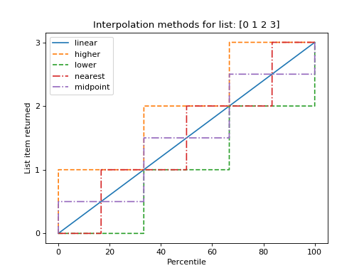
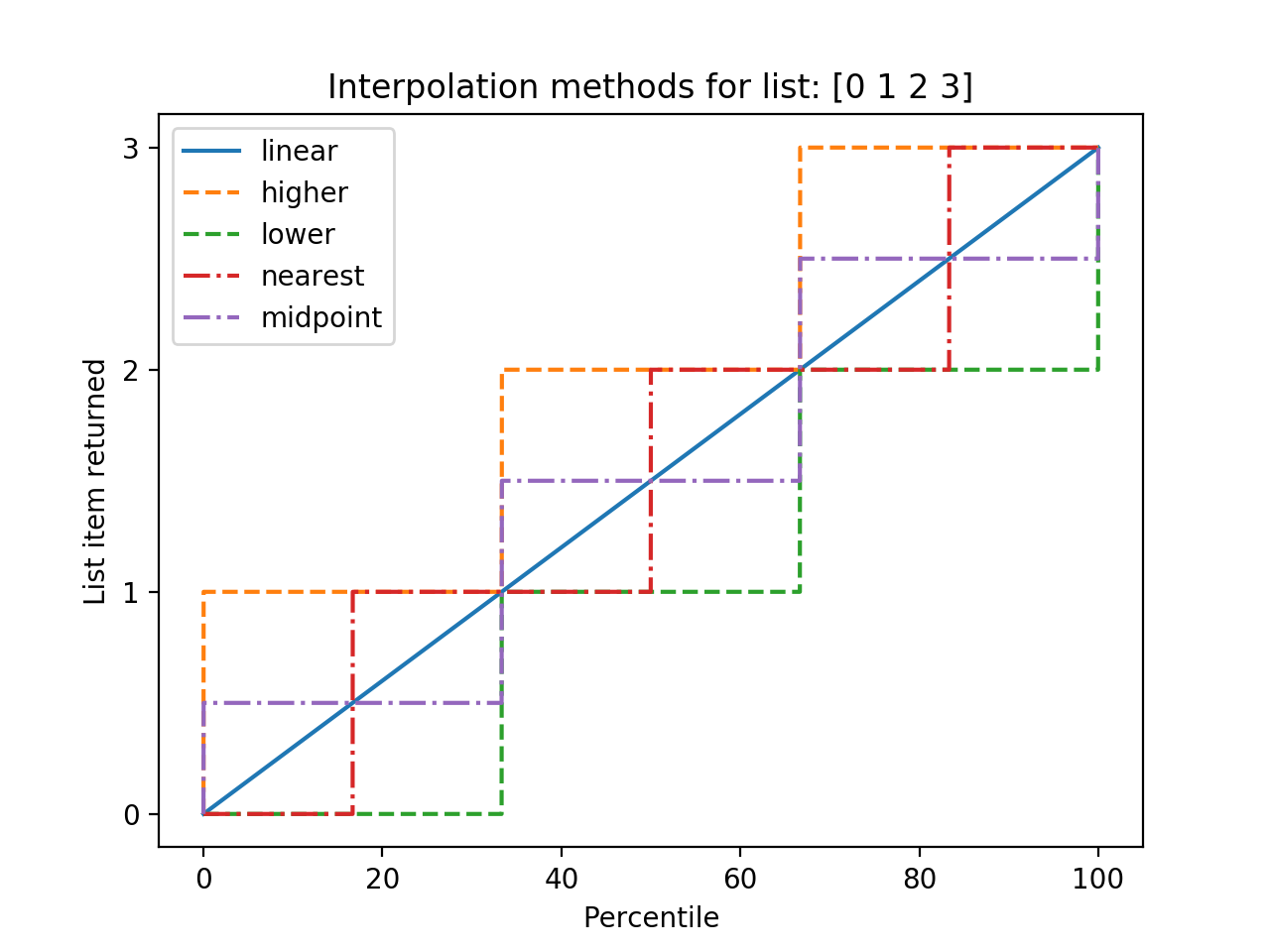
symjax.tensor.polyval(p, x)

Evaluate a polynomial at specific values.

LAX-backend implementation of polyval(). Original docstring below.

If p is of length N, this function returns the value:

p[0]*x**(N-1) + p[1]*x**(N-2) + ... + p[N-2]*x + p[N-1]

If x is a sequence, then p(x) is returned for each element of x. If x is another polynomial then the composite polynomial p(x(t)) is returned.

Parameters:

• p (array_like or poly1d object) –
• x (array_like or poly1d object) –

Returns:

values – If x is a poly1d instance, the result is the composition of the two polynomials, i.e., x is “substituted” in p and the simplified result is returned. In addition, the type of x - array_like or poly1d - governs the type of the output: x array_like => values array_like, x a poly1d object => values is also.

Return type:

ndarray or poly1d

See also

poly1d()

A polynomial class.

Notes

Horner’s scheme [1]_ is used to evaluate the polynomial. Even so, for polynomials of high degree the values may be inaccurate due to rounding errors. Use carefully.

If x is a subtype of ndarray the return value will be of the same type.

References

[1]	I. N. Bronshtein, K. A. Semendyayev, and K. A. Hirsch (Eng. trans. Ed.), Handbook of Mathematics, New York, Van Nostrand Reinhold Co., 1985, pg. 720.

Examples

>>> np.polyval([3,0,1], 5)  # 3 * 5**2 + 0 * 5**1 + 1
76
>>> np.polyval([3,0,1], np.poly1d(5))
poly1d([76.])
>>> np.polyval(np.poly1d([3,0,1]), 5)
76
>>> np.polyval(np.poly1d([3,0,1]), np.poly1d(5))
poly1d([76.])

symjax.tensor.power(x1, x2)

First array elements raised to powers from second array, element-wise.

LAX-backend implementation of power(). Original docstring below.

power(x1, x2, /, out=None, *, where=True, casting=’same_kind’, order=’K’, dtype=None, subok=True[, signature, extobj])

Raise each base in x1 to the positionally-corresponding power in x2. x1 and x2 must be broadcastable to the same shape. Note that an integer type raised to a negative integer power will raise a ValueError.

Parameters:

• x1 (array_like) – The bases.
• x2 (array_like) – The exponents. If x1.shape != x2.shape, they must be broadcastable to a common shape (which becomes the shape of the output).

Returns:

y – The bases in x1 raised to the exponents in x2. This is a scalar if both x1 and x2 are scalars.

Return type:

ndarray

See also

float_power()

power function that promotes integers to float

Examples

Cube each element in a list.

>>> x1 = range(6)
>>> x1
[0, 1, 2, 3, 4, 5]
>>> np.power(x1, 3)
array([  0,   1,   8,  27,  64, 125])

Raise the bases to different exponents.

>>> x2 = [1.0, 2.0, 3.0, 3.0, 2.0, 1.0]
>>> np.power(x1, x2)
array([  0.,   1.,   8.,  27.,  16.,   5.])

The effect of broadcasting.

>>> x2 = np.array([[1, 2, 3, 3, 2, 1], [1, 2, 3, 3, 2, 1]])
>>> x2
array([[1, 2, 3, 3, 2, 1],
       [1, 2, 3, 3, 2, 1]])
>>> np.power(x1, x2)
array([[ 0,  1,  8, 27, 16,  5],
       [ 0,  1,  8, 27, 16,  5]])

symjax.tensor.positive(x)

Numerical positive, element-wise.

LAX-backend implementation of positive(). Original docstring below.

positive(x, /, out=None, *, where=True, casting=’same_kind’, order=’K’, dtype=None, subok=True[, signature, extobj])

New in version 1.13.0.

Parameters:x (array_like or scalar) – Input array. Returns:y – Returned array or scalar: y = +x. This is a scalar if x is a scalar. Return type:ndarray or scalar

Notes

Equivalent to x.copy(), but only defined for types that support arithmetic.

symjax.tensor.prod(a, axis=None, dtype=None, out=None, keepdims=None, initial=None, where=None)

Return the product of array elements over a given axis.

LAX-backend implementation of prod(). Original docstring below.

Parameters:

• a (array_like) – Input data.
• axis (None or int or tuple of ints, optional) – Axis or axes along which a product is performed. The default, axis=None, will calculate the product of all the elements in the input array. If axis is negative it counts from the last to the first axis.
• dtype (dtype, optional) – The type of the returned array, as well as of the accumulator in which the elements are multiplied. The dtype of a is used by default unless a has an integer dtype of less precision than the default platform integer. In that case, if a is signed then the platform integer is used while if a is unsigned then an unsigned integer of the same precision as the platform integer is used.
• out (ndarray, optional) – Alternative output array in which to place the result. It must have the same shape as the expected output, but the type of the output values will be cast if necessary.
• keepdims (bool, optional) – If this is set to True, the axes which are reduced are left in the result as dimensions with size one. With this option, the result will broadcast correctly against the input array.
• initial (scalar, optional) – The starting value for this product. See ~numpy.ufunc.reduce for details.
• where (array_like of bool, optional) – Elements to include in the product. See ~numpy.ufunc.reduce for details.

Returns:

product_along_axis – An array shaped as a but with the specified axis removed. Returns a reference to out if specified.

Return type:

ndarray, see dtype parameter above.

See also

ndarray.prod()

equivalent method

ufuncs-output-type()

Notes

Arithmetic is modular when using integer types, and no error is raised on overflow. That means that, on a 32-bit platform:

>>> x = np.array([536870910, 536870910, 536870910, 536870910])
>>> np.prod(x)
16 # may vary

The product of an empty array is the neutral element 1:

>>> np.prod([])
1.0

Examples

By default, calculate the product of all elements:

>>> np.prod([1.,2.])
2.0

Even when the input array is two-dimensional:

>>> np.prod([[1.,2.],[3.,4.]])
24.0

But we can also specify the axis over which to multiply:

>>> np.prod([[1.,2.],[3.,4.]], axis=1)
array([  2.,  12.])

Or select specific elements to include:

>>> np.prod([1., np.nan, 3.], where=[True, False, True])
3.0

If the type of x is unsigned, then the output type is the unsigned platform integer:

>>> x = np.array([1, 2, 3], dtype=np.uint8)
>>> np.prod(x).dtype == np.uint
True

If x is of a signed integer type, then the output type is the default platform integer:

>>> x = np.array([1, 2, 3], dtype=np.int8)
>>> np.prod(x).dtype == int
True

You can also start the product with a value other than one:

>>> np.prod([1, 2], initial=5)
10

symjax.tensor.product(a, axis=None, dtype=None, out=None, keepdims=None, initial=None, where=None)

Return the product of array elements over a given axis.

LAX-backend implementation of prod(). Original docstring below.

Parameters:

• a (array_like) – Input data.
• axis (None or int or tuple of ints, optional) – Axis or axes along which a product is performed. The default, axis=None, will calculate the product of all the elements in the input array. If axis is negative it counts from the last to the first axis.
• dtype (dtype, optional) – The type of the returned array, as well as of the accumulator in which the elements are multiplied. The dtype of a is used by default unless a has an integer dtype of less precision than the default platform integer. In that case, if a is signed then the platform integer is used while if a is unsigned then an unsigned integer of the same precision as the platform integer is used.
• out (ndarray, optional) – Alternative output array in which to place the result. It must have the same shape as the expected output, but the type of the output values will be cast if necessary.
• keepdims (bool, optional) – If this is set to True, the axes which are reduced are left in the result as dimensions with size one. With this option, the result will broadcast correctly against the input array.
• initial (scalar, optional) – The starting value for this product. See ~numpy.ufunc.reduce for details.
• where (array_like of bool, optional) – Elements to include in the product. See ~numpy.ufunc.reduce for details.

Returns:

product_along_axis – An array shaped as a but with the specified axis removed. Returns a reference to out if specified.

Return type:

ndarray, see dtype parameter above.

See also

ndarray.prod()

equivalent method

ufuncs-output-type()

Notes

Arithmetic is modular when using integer types, and no error is raised on overflow. That means that, on a 32-bit platform:

>>> x = np.array([536870910, 536870910, 536870910, 536870910])
>>> np.prod(x)
16 # may vary

The product of an empty array is the neutral element 1:

>>> np.prod([])
1.0

Examples

By default, calculate the product of all elements:

>>> np.prod([1.,2.])
2.0

Even when the input array is two-dimensional:

>>> np.prod([[1.,2.],[3.,4.]])
24.0

But we can also specify the axis over which to multiply:

>>> np.prod([[1.,2.],[3.,4.]], axis=1)
array([  2.,  12.])

Or select specific elements to include:

>>> np.prod([1., np.nan, 3.], where=[True, False, True])
3.0

If the type of x is unsigned, then the output type is the unsigned platform integer:

>>> x = np.array([1, 2, 3], dtype=np.uint8)
>>> np.prod(x).dtype == np.uint
True

If x is of a signed integer type, then the output type is the default platform integer:

>>> x = np.array([1, 2, 3], dtype=np.int8)
>>> np.prod(x).dtype == int
True

You can also start the product with a value other than one:

>>> np.prod([1, 2], initial=5)
10

symjax.tensor.promote_types(a, b)

Returns the type to which a binary operation should cast its arguments.

For details of JAX’s type promotion semantics, see type-promotion.

Parameters:

• a – a numpy.dtype or a dtype specifier.
• b – a numpy.dtype or a dtype specifier.

Returns:

A numpy.dtype object.

symjax.tensor.ptp(a, axis=None, out=None, keepdims=False)

Range of values (maximum - minimum) along an axis.

LAX-backend implementation of ptp(). Original docstring below.

The name of the function comes from the acronym for ‘peak to peak’.

Warning

ptp preserves the data type of the array. This means the return value for an input of signed integers with n bits (e.g. np.int8, np.int16, etc) is also a signed integer with n bits. In that case, peak-to-peak values greater than 2**(n-1)-1 will be returned as negative values. An example with a work-around is shown below.

Parameters:

• a (array_like) – Input values.
• axis (None or int or tuple of ints, optional) – Axis along which to find the peaks. By default, flatten the array. axis may be negative, in which case it counts from the last to the first axis.
• out (array_like) – Alternative output array in which to place the result. It must have the same shape and buffer length as the expected output, but the type of the output values will be cast if necessary.
• keepdims (bool, optional) – If this is set to True, the axes which are reduced are left in the result as dimensions with size one. With this option, the result will broadcast correctly against the input array.

Returns:

ptp – A new array holding the result, unless out was specified, in which case a reference to out is returned.

Return type:

ndarray

Examples

>>> x = np.array([[4, 9, 2, 10],
...               [6, 9, 7, 12]])

>>> np.ptp(x, axis=1)
array([8, 6])

>>> np.ptp(x, axis=0)
array([2, 0, 5, 2])

>>> np.ptp(x)
10

This example shows that a negative value can be returned when the input is an array of signed integers.

>>> y = np.array([[1, 127],
...               [0, 127],
...               [-1, 127],
...               [-2, 127]], dtype=np.int8)
>>> np.ptp(y, axis=1)
array([ 126,  127, -128, -127], dtype=int8)

A work-around is to use the view() method to view the result as unsigned integers with the same bit width:

>>> np.ptp(y, axis=1).view(np.uint8)
array([126, 127, 128, 129], dtype=uint8)

symjax.tensor.quantile(a, q, axis=None, out=None, overwrite_input=False, interpolation='linear', keepdims=False)

Compute the q-th quantile of the data along the specified axis.

LAX-backend implementation of quantile(). Original docstring below.

New in version 1.15.0.

Parameters:

• a (array_like) – Input array or object that can be converted to an array.
• q (array_like of float) – Quantile or sequence of quantiles to compute, which must be between 0 and 1 inclusive.
• axis ({int, tuple of int, None}, optional) – Axis or axes along which the quantiles are computed. The default is to compute the quantile(s) along a flattened version of the array.
• out (ndarray, optional) – Alternative output array in which to place the result. It must have the same shape and buffer length as the expected output, but the type (of the output) will be cast if necessary.
• overwrite_input (bool, optional) – If True, then allow the input array a to be modified by intermediate calculations, to save memory. In this case, the contents of the input a after this function completes is undefined.
• interpolation ({'linear', 'lower', 'higher', 'midpoint', 'nearest'}) – This optional parameter specifies the interpolation method to use when the desired quantile lies between two data points i < j:
• keepdims (bool, optional) – If this is set to True, the axes which are reduced are left in the result as dimensions with size one. With this option, the result will broadcast correctly against the original array a.

Returns:

quantile – If q is a single quantile and axis=None, then the result is a scalar. If multiple quantiles are given, first axis of the result corresponds to the quantiles. The other axes are the axes that remain after the reduction of a. If the input contains integers or floats smaller than float64, the output data-type is float64. Otherwise, the output data-type is the same as that of the input. If out is specified, that array is returned instead.

Return type:

scalar or ndarray

See also

mean()

percentile()

equivalent to quantile, but with q in the range [0, 100].

median()

equivalent to quantile(..., 0.5)

nanquantile()

Notes

Given a vector V of length N, the q-th quantile of V is the value q of the way from the minimum to the maximum in a sorted copy of V. The values and distances of the two nearest neighbors as well as the interpolation parameter will determine the quantile if the normalized ranking does not match the location of q exactly. This function is the same as the median if q=0.5, the same as the minimum if q=0.0 and the same as the maximum if q=1.0.

Examples

>>> a = np.array([[10, 7, 4], [3, 2, 1]])
>>> a
array([[10,  7,  4],
       [ 3,  2,  1]])
>>> np.quantile(a, 0.5)
3.5
>>> np.quantile(a, 0.5, axis=0)
array([6.5, 4.5, 2.5])
>>> np.quantile(a, 0.5, axis=1)
array([7.,  2.])
>>> np.quantile(a, 0.5, axis=1, keepdims=True)
array([[7.],
       [2.]])
>>> m = np.quantile(a, 0.5, axis=0)
>>> out = np.zeros_like(m)
>>> np.quantile(a, 0.5, axis=0, out=out)
array([6.5, 4.5, 2.5])
>>> m
array([6.5, 4.5, 2.5])
>>> b = a.copy()
>>> np.quantile(b, 0.5, axis=1, overwrite_input=True)
array([7.,  2.])
>>> assert not np.all(a == b)

symjax.tensor.rad2deg(x)

Convert angles from radians to degrees.

LAX-backend implementation of rad2deg(). Original docstring below.

rad2deg(x, /, out=None, *, where=True, casting=’same_kind’, order=’K’, dtype=None, subok=True[, signature, extobj])

Parameters:x (array_like) – Angle in radians. Returns:y – The corresponding angle in degrees. This is a scalar if x is a scalar. Return type:ndarray

See also

deg2rad()

Convert angles from degrees to radians.

unwrap()

Remove large jumps in angle by wrapping.

Notes

New in version 1.3.0.

rad2deg(x) is 180 * x / pi.

Examples

>>> np.rad2deg(np.pi/2)
90.0

symjax.tensor.radians(x)

Convert angles from degrees to radians.

LAX-backend implementation of deg2rad(). Original docstring below.

deg2rad(x, /, out=None, *, where=True, casting=’same_kind’, order=’K’, dtype=None, subok=True[, signature, extobj])

Parameters:x (array_like) – Angles in degrees. Returns:y – The corresponding angle in radians. This is a scalar if x is a scalar. Return type:ndarray

See also

rad2deg()

Convert angles from radians to degrees.

unwrap()

Remove large jumps in angle by wrapping.

Notes

New in version 1.3.0.

deg2rad(x) is x * pi / 180.

Examples

>>> np.deg2rad(180)
3.1415926535897931

symjax.tensor.ravel(a, order='C')

Return a contiguous flattened array.

LAX-backend implementation of ravel(). Original docstring below.

A 1-D array, containing the elements of the input, is returned. A copy is made only if needed.

As of NumPy 1.10, the returned array will have the same type as the input array. (for example, a masked array will be returned for a masked array input)

Parameters:

• a (array_like) – Input array. The elements in a are read in the order specified by order, and packed as a 1-D array.
• order ({'C','F', 'A', 'K'}, optional) –

Returns:

y – y is an array of the same subtype as a, with shape (a.size,). Note that matrices are special cased for backward compatibility, if a is a matrix, then y is a 1-D ndarray.

Return type:

array_like

See also

ndarray.flat()

1-D iterator over an array.

ndarray.flatten()

1-D array copy of the elements of an array in row-major order.

ndarray.reshape()

Change the shape of an array without changing its data.

Notes

In row-major, C-style order, in two dimensions, the row index varies the slowest, and the column index the quickest. This can be generalized to multiple dimensions, where row-major order implies that the index along the first axis varies slowest, and the index along the last quickest. The opposite holds for column-major, Fortran-style index ordering.

When a view is desired in as many cases as possible, arr.reshape(-1) may be preferable.

Examples

It is equivalent to reshape(-1, order=order).

>>> x = np.array([[1, 2, 3], [4, 5, 6]])
>>> np.ravel(x)
array([1, 2, 3, 4, 5, 6])

>>> x.reshape(-1)
array([1, 2, 3, 4, 5, 6])

>>> np.ravel(x, order='F')
array([1, 4, 2, 5, 3, 6])

When order is ‘A’, it will preserve the array’s ‘C’ or ‘F’ ordering:

>>> np.ravel(x.T)
array([1, 4, 2, 5, 3, 6])
>>> np.ravel(x.T, order='A')
array([1, 2, 3, 4, 5, 6])

When order is ‘K’, it will preserve orderings that are neither ‘C’ nor ‘F’, but won’t reverse axes:

>>> a = np.arange(3)[::-1]; a
array([2, 1, 0])
>>> a.ravel(order='C')
array([2, 1, 0])
>>> a.ravel(order='K')
array([2, 1, 0])

>>> a = np.arange(12).reshape(2,3,2).swapaxes(1,2); a
array([[[ 0,  2,  4],
        [ 1,  3,  5]],
       [[ 6,  8, 10],
        [ 7,  9, 11]]])
>>> a.ravel(order='C')
array([ 0,  2,  4,  1,  3,  5,  6,  8, 10,  7,  9, 11])
>>> a.ravel(order='K')
array([ 0,  1,  2,  3,  4,  5,  6,  7,  8,  9, 10, 11])

symjax.tensor.real(val)

Return the real part of the complex argument.

LAX-backend implementation of real(). Original docstring below.

Parameters:val (array_like) – Input array. Returns:out – The real component of the complex argument. If val is real, the type of val is used for the output. If val has complex elements, the returned type is float. Return type:ndarray or scalar

See also

real_if_close(), imag(), angle()

Examples

>>> a = np.array([1+2j, 3+4j, 5+6j])
>>> a.real
array([1.,  3.,  5.])
>>> a.real = 9
>>> a
array([9.+2.j,  9.+4.j,  9.+6.j])
>>> a.real = np.array([9, 8, 7])
>>> a
array([9.+2.j,  8.+4.j,  7.+6.j])
>>> np.real(1 + 1j)
1.0

symjax.tensor.reciprocal(x)

Return the reciprocal of the argument, element-wise.

LAX-backend implementation of reciprocal(). Original docstring below.

reciprocal(x, /, out=None, *, where=True, casting=’same_kind’, order=’K’, dtype=None, subok=True[, signature, extobj])

Calculates 1/x.

Parameters:x (array_like) – Input array. Returns:y – Return array. This is a scalar if x is a scalar. Return type:ndarray

Notes

Note

This function is not designed to work with integers.

For integer arguments with absolute value larger than 1 the result is always zero because of the way Python handles integer division. For integer zero the result is an overflow.

Examples

>>> np.reciprocal(2.)
0.5
>>> np.reciprocal([1, 2., 3.33])
array([ 1.       ,  0.5      ,  0.3003003])

symjax.tensor.remainder(x1, x2)

Return element-wise remainder of division.

LAX-backend implementation of remainder(). Original docstring below.

remainder(x1, x2, /, out=None, *, where=True, casting=’same_kind’, order=’K’, dtype=None, subok=True[, signature, extobj])

Computes the remainder complementary to the floor_divide function. It is equivalent to the Python modulus operator``x1 % x2`` and has the same sign as the divisor x2. The MATLAB function equivalent to np.remainder is mod.

Warning

This should not be confused with:

• Python 3.7’s math.remainder and C’s remainder, which computes the IEEE remainder, which are the complement to round(x1 / x2).
• The MATLAB rem function and or the C % operator which is the complement to int(x1 / x2).

Parameters:

• x1 (array_like) – Dividend array.
• x2 (array_like) – Divisor array. If x1.shape != x2.shape, they must be broadcastable to a common shape (which becomes the shape of the output).

Returns:

y – The element-wise remainder of the quotient floor_divide(x1, x2). This is a scalar if both x1 and x2 are scalars.

Return type:

ndarray

See also

floor_divide()

Equivalent of Python // operator.

divmod()

Simultaneous floor division and remainder.

fmod()

Equivalent of the MATLAB rem function.

divide(), floor()

Notes

Returns 0 when x2 is 0 and both x1 and x2 are (arrays of) integers. mod is an alias of remainder.

Examples

>>> np.remainder([4, 7], [2, 3])
array([0, 1])
>>> np.remainder(np.arange(7), 5)
array([0, 1, 2, 3, 4, 0, 1])

symjax.tensor.repeat(a, repeats, axis=None, *, total_repeat_length=None)

Repeat elements of an array.

LAX-backend implementation of repeat(). Jax adds the optional total_repeat_length parameter which specifies the total number of repeat, and defaults to sum(repeats). It must be specified for repeat to be compilable. If sum(repeats) is larger than the specified total_repeat_length the remaining values will be discarded. In the case of sum(repeats) being smaller than the specified target length, the final value will be repeated.

Original docstring below.

Parameters:

• a (array_like) – Input array.
• repeats (int or array of ints) – The number of repetitions for each element. repeats is broadcasted to fit the shape of the given axis.
• axis (int, optional) – The axis along which to repeat values. By default, use the flattened input array, and return a flat output array.

Returns:

repeated_array – Output array which has the same shape as a, except along the given axis.

Return type:

ndarray

See also

tile()

Tile an array.

Examples

>>> np.repeat(3, 4)
array([3, 3, 3, 3])
>>> x = np.array([[1,2],[3,4]])
>>> np.repeat(x, 2)
array([1, 1, 2, 2, 3, 3, 4, 4])
>>> np.repeat(x, 3, axis=1)
array([[1, 1, 1, 2, 2, 2],
       [3, 3, 3, 4, 4, 4]])
>>> np.repeat(x, [1, 2], axis=0)
array([[1, 2],
       [3, 4],
       [3, 4]])

symjax.tensor.reshape(a, newshape, order='C')

Gives a new shape to an array without changing its data.

LAX-backend implementation of reshape(). Original docstring below.

Parameters:

• a (array_like) – Array to be reshaped.
• newshape (int or tuple of ints) – The new shape should be compatible with the original shape. If an integer, then the result will be a 1-D array of that length. One shape dimension can be -1. In this case, the value is inferred from the length of the array and remaining dimensions.
• order ({'C', 'F', 'A'}, optional) – Read the elements of a using this index order, and place the elements into the reshaped array using this index order. ‘C’ means to read / write the elements using C-like index order, with the last axis index changing fastest, back to the first axis index changing slowest. ‘F’ means to read / write the elements using Fortran-like index order, with the first index changing fastest, and the last index changing slowest. Note that the ‘C’ and ‘F’ options take no account of the memory layout of the underlying array, and only refer to the order of indexing. ‘A’ means to read / write the elements in Fortran-like index order if a is Fortran contiguous in memory, C-like order otherwise.

Returns:

reshaped_array – This will be a new view object if possible; otherwise, it will be a copy. Note there is no guarantee of the memory layout (C- or Fortran- contiguous) of the returned array.

Return type:

ndarray

See also

ndarray.reshape()

Equivalent method.

Notes

It is not always possible to change the shape of an array without copying the data. If you want an error to be raised when the data is copied, you should assign the new shape to the shape attribute of the array:

>>> a = np.zeros((10, 2))

# A transpose makes the array non-contiguous
>>> b = a.T

# Taking a view makes it possible to modify the shape without modifying
# the initial object.
>>> c = b.view()
>>> c.shape = (20)
Traceback (most recent call last):
   ...
AttributeError: Incompatible shape for in-place modification. Use
`.reshape()` to make a copy with the desired shape.

The order keyword gives the index ordering both for fetching the values from a, and then placing the values into the output array. For example, let’s say you have an array:

>>> a = np.arange(6).reshape((3, 2))
>>> a
array([[0, 1],
       [2, 3],
       [4, 5]])

You can think of reshaping as first raveling the array (using the given index order), then inserting the elements from the raveled array into the new array using the same kind of index ordering as was used for the raveling.

>>> np.reshape(a, (2, 3)) # C-like index ordering
array([[0, 1, 2],
       [3, 4, 5]])
>>> np.reshape(np.ravel(a), (2, 3)) # equivalent to C ravel then C reshape
array([[0, 1, 2],
       [3, 4, 5]])
>>> np.reshape(a, (2, 3), order='F') # Fortran-like index ordering
array([[0, 4, 3],
       [2, 1, 5]])
>>> np.reshape(np.ravel(a, order='F'), (2, 3), order='F')
array([[0, 4, 3],
       [2, 1, 5]])

Examples

>>> a = np.array([[1,2,3], [4,5,6]])
>>> np.reshape(a, 6)
array([1, 2, 3, 4, 5, 6])
>>> np.reshape(a, 6, order='F')
array([1, 4, 2, 5, 3, 6])

>>> np.reshape(a, (3,-1))       # the unspecified value is inferred to be 2
array([[1, 2],
       [3, 4],
       [5, 6]])

symjax.tensor.result_type(*args)

Returns the type that results from applying the NumPy

type promotion rules to the arguments.

LAX-backend implementation of result_type(). Original docstring below.

result_type(*arrays_and_dtypes)

Type promotion in NumPy works similarly to the rules in languages like C++, with some slight differences. When both scalars and arrays are used, the array’s type takes precedence and the actual value of the scalar is taken into account.

For example, calculating 3*a, where a is an array of 32-bit floats, intuitively should result in a 32-bit float output. If the 3 is a 32-bit integer, the NumPy rules indicate it can’t convert losslessly into a 32-bit float, so a 64-bit float should be the result type. By examining the value of the constant, ‘3’, we see that it fits in an 8-bit integer, which can be cast losslessly into the 32-bit float.

Returns

out : dtype

The result type.

dtype, promote_types, min_scalar_type, can_cast

New in version 1.6.0.

The specific algorithm used is as follows.

Categories are determined by first checking which of boolean, integer (int/uint), or floating point (float/complex) the maximum kind of all the arrays and the scalars are.

If there are only scalars or the maximum category of the scalars is higher than the maximum category of the arrays, the data types are combined with promote_types() to produce the return value.

Otherwise, min_scalar_type is called on each array, and the resulting data types are all combined with promote_types() to produce the return value.

The set of int values is not a subset of the uint values for types with the same number of bits, something not reflected in min_scalar_type(), but handled as a special case in result_type.

>>> np.result_type(3, np.arange(7, dtype='i1'))
dtype('int8')

>>> np.result_type('i4', 'c8')
dtype('complex128')

>>> np.result_type(3.0, -2)
dtype('float64')

symjax.tensor.right_shift(x1, x2)

Shift the bits of an integer to the right.

LAX-backend implementation of right_shift(). Original docstring below.

right_shift(x1, x2, /, out=None, *, where=True, casting=’same_kind’, order=’K’, dtype=None, subok=True[, signature, extobj])

Bits are shifted to the right x2. Because the internal representation of numbers is in binary format, this operation is equivalent to dividing x1 by 2**x2.

Parameters:

• x1 (array_like, int) – Input values.
• x2 (array_like, int) – Number of bits to remove at the right of x1. If x1.shape != x2.shape, they must be broadcastable to a common shape (which becomes the shape of the output).

Returns:

out – Return x1 with bits shifted x2 times to the right. This is a scalar if both x1 and x2 are scalars.

Return type:

ndarray, int

See also

left_shift()

Shift the bits of an integer to the left.

binary_repr()

Return the binary representation of the input number as a string.

Examples

>>> np.binary_repr(10)
'1010'
>>> np.right_shift(10, 1)
5
>>> np.binary_repr(5)
'101'

>>> np.right_shift(10, [1,2,3])
array([5, 2, 1])

symjax.tensor.roll(a, shift, axis=None)

Roll array elements along a given axis.

LAX-backend implementation of roll(). Original docstring below.

Elements that roll beyond the last position are re-introduced at the first.

Parameters:

• a (array_like) – Input array.
• shift (int or tuple of ints) – The number of places by which elements are shifted. If a tuple, then axis must be a tuple of the same size, and each of the given axes is shifted by the corresponding number. If an int while axis is a tuple of ints, then the same value is used for all given axes.
• axis (int or tuple of ints, optional) – Axis or axes along which elements are shifted. By default, the array is flattened before shifting, after which the original shape is restored.

Returns:

res – Output array, with the same shape as a.

Return type:

ndarray

See also

rollaxis()

Roll the specified axis backwards, until it lies in a given position.

Notes

New in version 1.12.0.

Supports rolling over multiple dimensions simultaneously.

Examples

>>> x = np.arange(10)
>>> np.roll(x, 2)
array([8, 9, 0, 1, 2, 3, 4, 5, 6, 7])
>>> np.roll(x, -2)
array([2, 3, 4, 5, 6, 7, 8, 9, 0, 1])

>>> x2 = np.reshape(x, (2,5))
>>> x2
array([[0, 1, 2, 3, 4],
       [5, 6, 7, 8, 9]])
>>> np.roll(x2, 1)
array([[9, 0, 1, 2, 3],
       [4, 5, 6, 7, 8]])
>>> np.roll(x2, -1)
array([[1, 2, 3, 4, 5],
       [6, 7, 8, 9, 0]])
>>> np.roll(x2, 1, axis=0)
array([[5, 6, 7, 8, 9],
       [0, 1, 2, 3, 4]])
>>> np.roll(x2, -1, axis=0)
array([[5, 6, 7, 8, 9],
       [0, 1, 2, 3, 4]])
>>> np.roll(x2, 1, axis=1)
array([[4, 0, 1, 2, 3],
       [9, 5, 6, 7, 8]])
>>> np.roll(x2, -1, axis=1)
array([[1, 2, 3, 4, 0],
       [6, 7, 8, 9, 5]])

symjax.tensor.rot90(m, k=1, axes=(0, 1))

Rotate an array by 90 degrees in the plane specified by axes.

LAX-backend implementation of rot90(). Original docstring below.

Rotation direction is from the first towards the second axis.

Parameters:

• m (array_like) – Array of two or more dimensions.
• k (integer) – Number of times the array is rotated by 90 degrees.

Returns:

y – A rotated view of m.

Return type:

ndarray

See also

flip()

Reverse the order of elements in an array along the given axis.

fliplr()

Flip an array horizontally.

flipud()

Flip an array vertically.

Notes

rot90(m, k=1, axes=(1,0)) is the reverse of rot90(m, k=1, axes=(0,1)) rot90(m, k=1, axes=(1,0)) is equivalent to rot90(m, k=-1, axes=(0,1))

Examples

>>> m = np.array([[1,2],[3,4]], int)
>>> m
array([[1, 2],
       [3, 4]])
>>> np.rot90(m)
array([[2, 4],
       [1, 3]])
>>> np.rot90(m, 2)
array([[4, 3],
       [2, 1]])
>>> m = np.arange(8).reshape((2,2,2))
>>> np.rot90(m, 1, (1,2))
array([[[1, 3],
        [0, 2]],
       [[5, 7],
        [4, 6]]])

symjax.tensor.round(a, decimals=0, out=None)

Round an array to the given number of decimals.

LAX-backend implementation of round_(). Original docstring below.

around : equivalent function; see for details.

symjax.tensor.row_stack(tup)

Stack arrays in sequence vertically (row wise).

LAX-backend implementation of vstack(). Original docstring below.

This is equivalent to concatenation along the first axis after 1-D arrays of shape (N,) have been reshaped to (1,N). Rebuilds arrays divided by vsplit.

This function makes most sense for arrays with up to 3 dimensions. For instance, for pixel-data with a height (first axis), width (second axis), and r/g/b channels (third axis). The functions concatenate, stack and block provide more general stacking and concatenation operations.

Parameters:tup (sequence of ndarrays) – The arrays must have the same shape along all but the first axis. 1-D arrays must have the same length. Returns:stacked – The array formed by stacking the given arrays, will be at least 2-D. Return type:ndarray

See also

concatenate()

Join a sequence of arrays along an existing axis.

stack()

Join a sequence of arrays along a new axis.

block()

Assemble an nd-array from nested lists of blocks.

hstack()

Stack arrays in sequence horizontally (column wise).

dstack()

Stack arrays in sequence depth wise (along third axis).

column_stack()

Stack 1-D arrays as columns into a 2-D array.

vsplit()

Split an array into multiple sub-arrays vertically (row-wise).

Examples

>>> a = np.array([1, 2, 3])
>>> b = np.array([2, 3, 4])
>>> np.vstack((a,b))
array([[1, 2, 3],
       [2, 3, 4]])

>>> a = np.array([[1], [2], [3]])
>>> b = np.array([[2], [3], [4]])
>>> np.vstack((a,b))
array([[1],
       [2],
       [3],
       [2],
       [3],
       [4]])

symjax.tensor.select(condlist, choicelist, default=0)

Return an array drawn from elements in choicelist, depending on conditions.

LAX-backend implementation of select(). Original docstring below.

Parameters:

• condlist (list of bool ndarrays) – The list of conditions which determine from which array in choicelist the output elements are taken. When multiple conditions are satisfied, the first one encountered in condlist is used.
• choicelist (list of ndarrays) – The list of arrays from which the output elements are taken. It has to be of the same length as condlist.
• default (scalar, optional) – The element inserted in output when all conditions evaluate to False.

Returns:

output – The output at position m is the m-th element of the array in choicelist where the m-th element of the corresponding array in condlist is True.

Return type:

ndarray

See also

where()

Return elements from one of two arrays depending on condition.

take(), choose(), compress(), diag(), diagonal()

Examples

>>> x = np.arange(10)
>>> condlist = [x<3, x>5]
>>> choicelist = [x, x**2]
>>> np.select(condlist, choicelist)
array([ 0,  1,  2, ..., 49, 64, 81])

symjax.tensor.sign(x)

Returns an element-wise indication of the sign of a number.

LAX-backend implementation of sign(). Original docstring below.

sign(x, /, out=None, *, where=True, casting=’same_kind’, order=’K’, dtype=None, subok=True[, signature, extobj])

The sign function returns -1 if x < 0, 0 if x==0, 1 if x > 0. nan is returned for nan inputs.

For complex inputs, the sign function returns sign(x.real) + 0j if x.real != 0 else sign(x.imag) + 0j.

complex(nan, 0) is returned for complex nan inputs.

Parameters:x (array_like) – Input values. Returns:y – The sign of x. This is a scalar if x is a scalar. Return type:ndarray

Notes

There is more than one definition of sign in common use for complex numbers. The definition used here is equivalent to \(x/\sqrt{x*x}\) which is different from a common alternative, \(x/|x|\).

Examples

>>> np.sign([-5., 4.5])
array([-1.,  1.])
>>> np.sign(0)
0
>>> np.sign(5-2j)
(1+0j)

symjax.tensor.signbit(x)

Returns element-wise True where signbit is set (less than zero).

LAX-backend implementation of signbit(). Original docstring below.

signbit(x, /, out=None, *, where=True, casting=’same_kind’, order=’K’, dtype=None, subok=True[, signature, extobj])

Parameters:x (array_like) – The input value(s). Returns:result – Output array, or reference to out if that was supplied. This is a scalar if x is a scalar. Return type:ndarray of bool

Examples

>>> np.signbit(-1.2)
True
>>> np.signbit(np.array([1, -2.3, 2.1]))
array([False,  True, False])

symjax.tensor.sin(x)

Trigonometric sine, element-wise.

LAX-backend implementation of sin(). Original docstring below.

sin(x, /, out=None, *, where=True, casting=’same_kind’, order=’K’, dtype=None, subok=True[, signature, extobj])

Parameters:x (array_like) – Angle, in radians (\(2 \pi\) rad equals 360 degrees). Returns:y – The sine of each element of x. This is a scalar if x is a scalar. Return type:array_like

See also

arcsin(), sinh(), cos()

Notes

The sine is one of the fundamental functions of trigonometry (the mathematical study of triangles). Consider a circle of radius 1 centered on the origin. A ray comes in from the \(+x\) axis, makes an angle at the origin (measured counter-clockwise from that axis), and departs from the origin. The \(y\) coordinate of the outgoing ray’s intersection with the unit circle is the sine of that angle. It ranges from -1 for \(x=3\pi / 2\) to +1 for \(\pi / 2.\) The function has zeroes where the angle is a multiple of \(\pi\). Sines of angles between \(\pi\) and \(2\pi\) are negative. The numerous properties of the sine and related functions are included in any standard trigonometry text.

Examples

Print sine of one angle:

>>> np.sin(np.pi/2.)
1.0

Print sines of an array of angles given in degrees:

>>> np.sin(np.array((0., 30., 45., 60., 90.)) * np.pi / 180. )
array([ 0.        ,  0.5       ,  0.70710678,  0.8660254 ,  1.        ])

Plot the sine function:

>>> import matplotlib.pylab as plt
>>> x = np.linspace(-np.pi, np.pi, 201)
>>> plt.plot(x, np.sin(x))
>>> plt.xlabel('Angle [rad]')
>>> plt.ylabel('sin(x)')
>>> plt.axis('tight')
>>> plt.show()

symjax.tensor.sinc(x)

Return the sinc function.

LAX-backend implementation of sinc(). Original docstring below.

The sinc function is \(\sin(\pi x)/(\pi x)\).

x : ndarray

Array (possibly multi-dimensional) of values for which to to calculate sinc(x).

out : ndarray

sinc(x), which has the same shape as the input.

sinc(0) is the limit value 1.

The name sinc is short for “sine cardinal” or “sinus cardinalis”.

The sinc function is used in various signal processing applications, including in anti-aliasing, in the construction of a Lanczos resampling filter, and in interpolation.

For bandlimited interpolation of discrete-time signals, the ideal interpolation kernel is proportional to the sinc function.

[1]	Weisstein, Eric W. “Sinc Function.” From MathWorld–A Wolfram Web Resource. http://mathworld.wolfram.com/SincFunction.html

[2]	Wikipedia, “Sinc function”, https://en.wikipedia.org/wiki/Sinc_function

>>> import matplotlib.pyplot as plt
>>> x = np.linspace(-4, 4, 41)
>>> np.sinc(x)
 array([-3.89804309e-17,  -4.92362781e-02,  -8.40918587e-02, # may vary
        -8.90384387e-02,  -5.84680802e-02,   3.89804309e-17,
        6.68206631e-02,   1.16434881e-01,   1.26137788e-01,
        8.50444803e-02,  -3.89804309e-17,  -1.03943254e-01,
        -1.89206682e-01,  -2.16236208e-01,  -1.55914881e-01,
        3.89804309e-17,   2.33872321e-01,   5.04551152e-01,
        7.56826729e-01,   9.35489284e-01,   1.00000000e+00,
        9.35489284e-01,   7.56826729e-01,   5.04551152e-01,
        2.33872321e-01,   3.89804309e-17,  -1.55914881e-01,
       -2.16236208e-01,  -1.89206682e-01,  -1.03943254e-01,
       -3.89804309e-17,   8.50444803e-02,   1.26137788e-01,
        1.16434881e-01,   6.68206631e-02,   3.89804309e-17,
        -5.84680802e-02,  -8.90384387e-02,  -8.40918587e-02,
        -4.92362781e-02,  -3.89804309e-17])

>>> plt.plot(x, np.sinc(x))
[<matplotlib.lines.Line2D object at 0x...>]
>>> plt.title("Sinc Function")
Text(0.5, 1.0, 'Sinc Function')
>>> plt.ylabel("Amplitude")
Text(0, 0.5, 'Amplitude')
>>> plt.xlabel("X")
Text(0.5, 0, 'X')
>>> plt.show()

symjax.tensor.sinh(x)

Hyperbolic sine, element-wise.

LAX-backend implementation of sinh(). Original docstring below.

sinh(x, /, out=None, *, where=True, casting=’same_kind’, order=’K’, dtype=None, subok=True[, signature, extobj])

Equivalent to 1/2 * (np.exp(x) - np.exp(-x)) or -1j * np.sin(1j*x).

Parameters:x (array_like) – Input array. Returns:y – The corresponding hyperbolic sine values. This is a scalar if x is a scalar. Return type:ndarray

Notes

If out is provided, the function writes the result into it, and returns a reference to out. (See Examples)

References

M. Abramowitz and I. A. Stegun, Handbook of Mathematical Functions. New York, NY: Dover, 1972, pg. 83.

Examples

>>> np.sinh(0)
0.0
>>> np.sinh(np.pi*1j/2)
1j
>>> np.sinh(np.pi*1j) # (exact value is 0)
1.2246063538223773e-016j
>>> # Discrepancy due to vagaries of floating point arithmetic.

>>> # Example of providing the optional output parameter
>>> out1 = np.array([0], dtype='d')
>>> out2 = np.sinh([0.1], out1)
>>> out2 is out1
True

>>> # Example of ValueError due to provision of shape mis-matched `out`
>>> np.sinh(np.zeros((3,3)),np.zeros((2,2)))
Traceback (most recent call last):
  File "<stdin>", line 1, in <module>
ValueError: operands could not be broadcast together with shapes (3,3) (2,2)

symjax.tensor.sometrue(a, axis=None, out=None, keepdims=None)

Test whether any array element along a given axis evaluates to True.

LAX-backend implementation of any(). Original docstring below.

Returns single boolean unless axis is not None

Parameters:

• a (array_like) – Input array or object that can be converted to an array.
• axis (None or int or tuple of ints, optional) – Axis or axes along which a logical OR reduction is performed. The default (axis=None) is to perform a logical OR over all the dimensions of the input array. axis may be negative, in which case it counts from the last to the first axis.
• out (ndarray, optional) – Alternate output array in which to place the result. It must have the same shape as the expected output and its type is preserved (e.g., if it is of type float, then it will remain so, returning 1.0 for True and 0.0 for False, regardless of the type of a). See ufuncs-output-type for more details.
• keepdims (bool, optional) – If this is set to True, the axes which are reduced are left in the result as dimensions with size one. With this option, the result will broadcast correctly against the input array.

Returns:

any – A new boolean or ndarray is returned unless out is specified, in which case a reference to out is returned.

Return type:

bool or ndarray

See also

ndarray.any()

equivalent method

all()

Test whether all elements along a given axis evaluate to True.

Notes

Not a Number (NaN), positive infinity and negative infinity evaluate to True because these are not equal to zero.

Examples

>>> np.any([[True, False], [True, True]])
True

>>> np.any([[True, False], [False, False]], axis=0)
array([ True, False])

>>> np.any([-1, 0, 5])
True

>>> np.any(np.nan)
True

>>> o=np.array(False)
>>> z=np.any([-1, 4, 5], out=o)
>>> z, o
(array(True), array(True))
>>> # Check now that z is a reference to o
>>> z is o
True
>>> id(z), id(o) # identity of z and o              # doctest: +SKIP
(191614240, 191614240)

symjax.tensor.sort(a, axis=-1, kind='quicksort', order=None)

Return a sorted copy of an array.

LAX-backend implementation of sort(). Original docstring below.

Parameters:

• a (array_like) – Array to be sorted.
• axis (int or None, optional) – Axis along which to sort. If None, the array is flattened before sorting. The default is -1, which sorts along the last axis.
• kind ({'quicksort', 'mergesort', 'heapsort', 'stable'}, optional) – Sorting algorithm. The default is ‘quicksort’. Note that both ‘stable’ and ‘mergesort’ use timsort or radix sort under the covers and, in general, the actual implementation will vary with data type. The ‘mergesort’ option is retained for backwards compatibility.
• order (str or list of str, optional) – When a is an array with fields defined, this argument specifies which fields to compare first, second, etc. A single field can be specified as a string, and not all fields need be specified, but unspecified fields will still be used, in the order in which they come up in the dtype, to break ties.

Returns:

sorted_array – Array of the same type and shape as a.

Return type:

ndarray

See also

ndarray.sort()

Method to sort an array in-place.

argsort()

Indirect sort.

lexsort()

Indirect stable sort on multiple keys.

searchsorted()

Find elements in a sorted array.

partition()

Partial sort.

Notes

The various sorting algorithms are characterized by their average speed, worst case performance, work space size, and whether they are stable. A stable sort keeps items with the same key in the same relative order. The four algorithms implemented in NumPy have the following properties:

kind	speed	worst case	work space	stable
‘quicksort’	1	O(n^2)	0	no
‘heapsort’	3	O(n*log(n))	0	no
‘mergesort’	2	O(n*log(n))	~n/2	yes
‘timsort’	2	O(n*log(n))	~n/2	yes

Note

The datatype determines which of ‘mergesort’ or ‘timsort’ is actually used, even if ‘mergesort’ is specified. User selection at a finer scale is not currently available.

All the sort algorithms make temporary copies of the data when sorting along any but the last axis. Consequently, sorting along the last axis is faster and uses less space than sorting along any other axis.

The sort order for complex numbers is lexicographic. If both the real and imaginary parts are non-nan then the order is determined by the real parts except when they are equal, in which case the order is determined by the imaginary parts.

Previous to numpy 1.4.0 sorting real and complex arrays containing nan values led to undefined behaviour. In numpy versions >= 1.4.0 nan values are sorted to the end. The extended sort order is:

• Real: [R, nan]
• Complex: [R + Rj, R + nanj, nan + Rj, nan + nanj]

where R is a non-nan real value. Complex values with the same nan placements are sorted according to the non-nan part if it exists. Non-nan values are sorted as before.

New in version 1.12.0.

quicksort has been changed to introsort. When sorting does not make enough progress it switches to heapsort. This implementation makes quicksort O(n*log(n)) in the worst case.

‘stable’ automatically chooses the best stable sorting algorithm for the data type being sorted. It, along with ‘mergesort’ is currently mapped to timsort or radix sort depending on the data type. API forward compatibility currently limits the ability to select the implementation and it is hardwired for the different data types.

New in version 1.17.0.

Timsort is added for better performance on already or nearly sorted data. On random data timsort is almost identical to mergesort. It is now used for stable sort while quicksort is still the default sort if none is chosen. For timsort details, refer to CPython listsort.txt. ‘mergesort’ and ‘stable’ are mapped to radix sort for integer data types. Radix sort is an O(n) sort instead of O(n log n).

Changed in version 1.18.0.

NaT now sorts to the end of arrays for consistency with NaN.

Examples

>>> a = np.array([[1,4],[3,1]])
>>> np.sort(a)                # sort along the last axis
array([[1, 4],
       [1, 3]])
>>> np.sort(a, axis=None)     # sort the flattened array
array([1, 1, 3, 4])
>>> np.sort(a, axis=0)        # sort along the first axis
array([[1, 1],
       [3, 4]])

Use the order keyword to specify a field to use when sorting a structured array:

>>> dtype = [('name', 'S10'), ('height', float), ('age', int)]
>>> values = [('Arthur', 1.8, 41), ('Lancelot', 1.9, 38),
...           ('Galahad', 1.7, 38)]
>>> a = np.array(values, dtype=dtype)       # create a structured array
>>> np.sort(a, order='height')                        # doctest: +SKIP
array([('Galahad', 1.7, 38), ('Arthur', 1.8, 41),
       ('Lancelot', 1.8999999999999999, 38)],
      dtype=[('name', '|S10'), ('height', '<f8'), ('age', '<i4')])

Sort by age, then height if ages are equal:

>>> np.sort(a, order=['age', 'height'])               # doctest: +SKIP
array([('Galahad', 1.7, 38), ('Lancelot', 1.8999999999999999, 38),
       ('Arthur', 1.8, 41)],
      dtype=[('name', '|S10'), ('height', '<f8'), ('age', '<i4')])

symjax.tensor.split(ary, indices_or_sections, axis=0)

Split an array into multiple sub-arrays as views into ary.

LAX-backend implementation of split(). Original docstring below.

Parameters:

• ary (ndarray) – Array to be divided into sub-arrays.
• indices_or_sections (int or 1-D array) – If indices_or_sections is an integer, N, the array will be divided into N equal arrays along axis. If such a split is not possible, an error is raised.
• axis (int, optional) – The axis along which to split, default is 0.

Returns:

sub-arrays – A list of sub-arrays as views into ary.

Return type:

list of ndarrays

Raises:

ValueError – If indices_or_sections is given as an integer, but a split does not result in equal division.

See also

array_split()

Split an array into multiple sub-arrays of equal or near-equal size. Does not raise an exception if an equal division cannot be made.

hsplit()

Split array into multiple sub-arrays horizontally (column-wise).

vsplit()

Split array into multiple sub-arrays vertically (row wise).

dsplit()

Split array into multiple sub-arrays along the 3rd axis (depth).

concatenate()

Join a sequence of arrays along an existing axis.

stack()

Join a sequence of arrays along a new axis.

hstack()

Stack arrays in sequence horizontally (column wise).

vstack()

Stack arrays in sequence vertically (row wise).

dstack()

Stack arrays in sequence depth wise (along third dimension).

Examples

>>> x = np.arange(9.0)
>>> np.split(x, 3)
[array([0.,  1.,  2.]), array([3.,  4.,  5.]), array([6.,  7.,  8.])]

>>> x = np.arange(8.0)
>>> np.split(x, [3, 5, 6, 10])
[array([0.,  1.,  2.]),
 array([3.,  4.]),
 array([5.]),
 array([6.,  7.]),
 array([], dtype=float64)]

symjax.tensor.sqrt(x)

Return the non-negative square-root of an array, element-wise.

LAX-backend implementation of sqrt(). Original docstring below.

sqrt(x, /, out=None, *, where=True, casting=’same_kind’, order=’K’, dtype=None, subok=True[, signature, extobj])

Parameters:x (array_like) – The values whose square-roots are required. Returns:y – An array of the same shape as x, containing the positive square-root of each element in x. If any element in x is complex, a complex array is returned (and the square-roots of negative reals are calculated). If all of the elements in x are real, so is y, with negative elements returning nan. If out was provided, y is a reference to it. This is a scalar if x is a scalar. Return type:ndarray

See also

lib.scimath.sqrt()

A version which returns complex numbers when given negative reals.

Notes

sqrt has–consistent with common convention–as its branch cut the real “interval” [-inf, 0), and is continuous from above on it. A branch cut is a curve in the complex plane across which a given complex function fails to be continuous.

Examples

>>> np.sqrt([1,4,9])
array([ 1.,  2.,  3.])

>>> np.sqrt([4, -1, -3+4J])
array([ 2.+0.j,  0.+1.j,  1.+2.j])

>>> np.sqrt([4, -1, np.inf])
array([ 2., nan, inf])

symjax.tensor.square(x)

Return the element-wise square of the input.

LAX-backend implementation of square(). Original docstring below.

square(x, /, out=None, *, where=True, casting=’same_kind’, order=’K’, dtype=None, subok=True[, signature, extobj])

Parameters:x (array_like) – Input data. Returns:out – Element-wise x*x, of the same shape and dtype as x. This is a scalar if x is a scalar. Return type:ndarray or scalar

See also

numpy.linalg.matrix_power(), sqrt(), power()

Examples

>>> np.square([-1j, 1])
array([-1.-0.j,  1.+0.j])

symjax.tensor.squeeze(a, axis: Union[int, Tuple[int, ...]] = None)

Remove single-dimensional entries from the shape of an array.

LAX-backend implementation of squeeze(). Original docstring below.

Parameters:

• a (array_like) – Input data.
• axis (None or int or tuple of ints, optional) –

  New in version 1.7.0.

Returns:

squeezed – The input array, but with all or a subset of the dimensions of length 1 removed. This is always a itself or a view into a. Note that if all axes are squeezed, the result is a 0d array and not a scalar.

Return type:

ndarray

Raises:

ValueError – If axis is not None, and an axis being squeezed is not of length 1

See also

expand_dims()

The inverse operation, adding singleton dimensions

reshape()

Insert, remove, and combine dimensions, and resize existing ones

Examples

>>> x = np.array([[[0], [1], [2]]])
>>> x.shape
(1, 3, 1)
>>> np.squeeze(x).shape
(3,)
>>> np.squeeze(x, axis=0).shape
(3, 1)
>>> np.squeeze(x, axis=1).shape
Traceback (most recent call last):
...
ValueError: cannot select an axis to squeeze out which has size not equal to one
>>> np.squeeze(x, axis=2).shape
(1, 3)
>>> x = np.array([[1234]])
>>> x.shape
(1, 1)
>>> np.squeeze(x)
array(1234)  # 0d array
>>> np.squeeze(x).shape
()
>>> np.squeeze(x)[()]
1234

symjax.tensor.stack(arrays, axis=0, out=None)

Join a sequence of arrays along a new axis.

LAX-backend implementation of stack(). Original docstring below.

The axis parameter specifies the index of the new axis in the dimensions of the result. For example, if axis=0 it will be the first dimension and if axis=-1 it will be the last dimension.

New in version 1.10.0.

Parameters:

• arrays (sequence of array_like) – Each array must have the same shape.
• axis (int, optional) – The axis in the result array along which the input arrays are stacked.
• out (ndarray, optional) – If provided, the destination to place the result. The shape must be correct, matching that of what stack would have returned if no out argument were specified.

Returns:

stacked – The stacked array has one more dimension than the input arrays.

Return type:

ndarray

See also

concatenate()

Join a sequence of arrays along an existing axis.

block()

Assemble an nd-array from nested lists of blocks.

split()

Split array into a list of multiple sub-arrays of equal size.

Examples

>>> arrays = [np.random.randn(3, 4) for _ in range(10)]
>>> np.stack(arrays, axis=0).shape
(10, 3, 4)

>>> np.stack(arrays, axis=1).shape
(3, 10, 4)

>>> np.stack(arrays, axis=2).shape
(3, 4, 10)

>>> a = np.array([1, 2, 3])
>>> b = np.array([2, 3, 4])
>>> np.stack((a, b))
array([[1, 2, 3],
       [2, 3, 4]])

>>> np.stack((a, b), axis=-1)
array([[1, 2],
       [2, 3],
       [3, 4]])

symjax.tensor.std(a, axis=None, dtype=None, out=None, ddof=0, keepdims=False)

Compute the standard deviation along the specified axis.

LAX-backend implementation of std(). Original docstring below.

Returns the standard deviation, a measure of the spread of a distribution, of the array elements. The standard deviation is computed for the flattened array by default, otherwise over the specified axis.

Parameters:

• a (array_like) – Calculate the standard deviation of these values.
• axis (None or int or tuple of ints, optional) – Axis or axes along which the standard deviation is computed. The default is to compute the standard deviation of the flattened array.
• dtype (dtype, optional) – Type to use in computing the standard deviation. For arrays of integer type the default is float64, for arrays of float types it is the same as the array type.
• out (ndarray, optional) – Alternative output array in which to place the result. It must have the same shape as the expected output but the type (of the calculated values) will be cast if necessary.
• ddof (int, optional) – Means Delta Degrees of Freedom. The divisor used in calculations is N - ddof, where N represents the number of elements. By default ddof is zero.
• keepdims (bool, optional) – If this is set to True, the axes which are reduced are left in the result as dimensions with size one. With this option, the result will broadcast correctly against the input array.

Returns:

standard_deviation – If out is None, return a new array containing the standard deviation, otherwise return a reference to the output array.

Return type:

ndarray, see dtype parameter above.

See also

var(), mean(), nanmean(), nanstd(), nanvar(), ufuncs-output-type()

Notes

The standard deviation is the square root of the average of the squared deviations from the mean, i.e., std = sqrt(mean(abs(x - x.mean())**2)).

The average squared deviation is normally calculated as x.sum() / N, where N = len(x). If, however, ddof is specified, the divisor N - ddof is used instead. In standard statistical practice, ddof=1 provides an unbiased estimator of the variance of the infinite population. ddof=0 provides a maximum likelihood estimate of the variance for normally distributed variables. The standard deviation computed in this function is the square root of the estimated variance, so even with ddof=1, it will not be an unbiased estimate of the standard deviation per se.

Note that, for complex numbers, std takes the absolute value before squaring, so that the result is always real and nonnegative.

For floating-point input, the std is computed using the same precision the input has. Depending on the input data, this can cause the results to be inaccurate, especially for float32 (see example below). Specifying a higher-accuracy accumulator using the dtype keyword can alleviate this issue.

Examples

>>> a = np.array([[1, 2], [3, 4]])
>>> np.std(a)
1.1180339887498949 # may vary
>>> np.std(a, axis=0)
array([1.,  1.])
>>> np.std(a, axis=1)
array([0.5,  0.5])

In single precision, std() can be inaccurate:

>>> a = np.zeros((2, 512*512), dtype=np.float32)
>>> a[0, :] = 1.0
>>> a[1, :] = 0.1
>>> np.std(a)
0.45000005

Computing the standard deviation in float64 is more accurate:

>>> np.std(a, dtype=np.float64)
0.44999999925494177 # may vary

symjax.tensor.subtract(x1, x2)

Subtract arguments, element-wise.

LAX-backend implementation of subtract(). Original docstring below.

subtract(x1, x2, /, out=None, *, where=True, casting=’same_kind’, order=’K’, dtype=None, subok=True[, signature, extobj])

Parameters:x2 (x1,) – The arrays to be subtracted from each other. If x1.shape != x2.shape, they must be broadcastable to a common shape (which becomes the shape of the output). Returns:y – The difference of x1 and x2, element-wise. This is a scalar if both x1 and x2 are scalars. Return type:ndarray

Notes

Equivalent to x1 - x2 in terms of array broadcasting.

Examples

>>> np.subtract(1.0, 4.0)
-3.0

>>> x1 = np.arange(9.0).reshape((3, 3))
>>> x2 = np.arange(3.0)
>>> np.subtract(x1, x2)
array([[ 0.,  0.,  0.],
       [ 3.,  3.,  3.],
       [ 6.,  6.,  6.]])

symjax.tensor.sum(a, axis=None, dtype=None, out=None, keepdims=None, initial=None, where=None)

Sum of array elements over a given axis.

LAX-backend implementation of sum(). Original docstring below.

Parameters:

• a (array_like) – Elements to sum.
• axis (None or int or tuple of ints, optional) – Axis or axes along which a sum is performed. The default, axis=None, will sum all of the elements of the input array. If axis is negative it counts from the last to the first axis.
• dtype (dtype, optional) – The type of the returned array and of the accumulator in which the elements are summed. The dtype of a is used by default unless a has an integer dtype of less precision than the default platform integer. In that case, if a is signed then the platform integer is used while if a is unsigned then an unsigned integer of the same precision as the platform integer is used.
• out (ndarray, optional) – Alternative output array in which to place the result. It must have the same shape as the expected output, but the type of the output values will be cast if necessary.
• keepdims (bool, optional) – If this is set to True, the axes which are reduced are left in the result as dimensions with size one. With this option, the result will broadcast correctly against the input array.
• initial (scalar, optional) – Starting value for the sum. See ~numpy.ufunc.reduce for details.
• where (array_like of bool, optional) – Elements to include in the sum. See ~numpy.ufunc.reduce for details.

Returns:

sum_along_axis – An array with the same shape as a, with the specified axis removed. If a is a 0-d array, or if axis is None, a scalar is returned. If an output array is specified, a reference to out is returned.

Return type:

ndarray

See also

ndarray.sum()

Equivalent method.

add.reduce()

Equivalent functionality of add.

cumsum()

Cumulative sum of array elements.

trapz()

Integration of array values using the composite trapezoidal rule.

mean(), average()

Notes

Arithmetic is modular when using integer types, and no error is raised on overflow.

The sum of an empty array is the neutral element 0:

>>> np.sum([])
0.0

For floating point numbers the numerical precision of sum (and np.add.reduce) is in general limited by directly adding each number individually to the result causing rounding errors in every step. However, often numpy will use a numerically better approach (partial pairwise summation) leading to improved precision in many use-cases. This improved precision is always provided when no axis is given. When axis is given, it will depend on which axis is summed. Technically, to provide the best speed possible, the improved precision is only used when the summation is along the fast axis in memory. Note that the exact precision may vary depending on other parameters. In contrast to NumPy, Python’s math.fsum function uses a slower but more precise approach to summation. Especially when summing a large number of lower precision floating point numbers, such as float32, numerical errors can become significant. In such cases it can be advisable to use dtype=”float64” to use a higher precision for the output.

Examples

>>> np.sum([0.5, 1.5])
2.0
>>> np.sum([0.5, 0.7, 0.2, 1.5], dtype=np.int32)
1
>>> np.sum([[0, 1], [0, 5]])
6
>>> np.sum([[0, 1], [0, 5]], axis=0)
array([0, 6])
>>> np.sum([[0, 1], [0, 5]], axis=1)
array([1, 5])
>>> np.sum([[0, 1], [np.nan, 5]], where=[False, True], axis=1)
array([1., 5.])

If the accumulator is too small, overflow occurs:

>>> np.ones(128, dtype=np.int8).sum(dtype=np.int8)
-128

You can also start the sum with a value other than zero:

>>> np.sum([10], initial=5)
15

symjax.tensor.swapaxes(a, axis1, axis2)

Interchange two axes of an array.

LAX-backend implementation of swapaxes(). Original docstring below.

Parameters:

• a (array_like) – Input array.
• axis1 (int) – First axis.
• axis2 (int) – Second axis.

Returns:

a_swapped – For NumPy >= 1.10.0, if a is an ndarray, then a view of a is returned; otherwise a new array is created. For earlier NumPy versions a view of a is returned only if the order of the axes is changed, otherwise the input array is returned.

Return type:

ndarray

Examples

>>> x = np.array([[1,2,3]])
>>> np.swapaxes(x,0,1)
array([[1],
       [2],
       [3]])

>>> x = np.array([[[0,1],[2,3]],[[4,5],[6,7]]])
>>> x
array([[[0, 1],
        [2, 3]],
       [[4, 5],
        [6, 7]]])

>>> np.swapaxes(x,0,2)
array([[[0, 4],
        [2, 6]],
       [[1, 5],
        [3, 7]]])

symjax.tensor.take(a, indices, axis=None, out=None, mode=None)

Take elements from an array along an axis.

LAX-backend implementation of take(). Original docstring below.

When axis is not None, this function does the same thing as “fancy” indexing (indexing arrays using arrays); however, it can be easier to use if you need elements along a given axis. A call such as np.take(arr, indices, axis=3) is equivalent to arr[:,:,:,indices,...].

Explained without fancy indexing, this is equivalent to the following use of ndindex, which sets each of ii, jj, and kk to a tuple of indices:

Ni, Nk = a.shape[:axis], a.shape[axis+1:]
Nj = indices.shape
for ii in ndindex(Ni):
    for jj in ndindex(Nj):
        for kk in ndindex(Nk):
            out[ii + jj + kk] = a[ii + (indices[jj],) + kk]

Parameters:

• a (array_like (Ni..., M, Nk...)) – The source array.
• indices (array_like (Nj...)) – The indices of the values to extract.
• axis (int, optional) – The axis over which to select values. By default, the flattened input array is used.
• out (ndarray, optional (Ni..., Nj..., Nk...)) – If provided, the result will be placed in this array. It should be of the appropriate shape and dtype. Note that out is always buffered if mode=’raise’; use other modes for better performance.
• mode ({'raise', 'wrap', 'clip'}, optional) – Specifies how out-of-bounds indices will behave.

Returns:

out – The returned array has the same type as a.

Return type:

ndarray (Ni…, Nj…, Nk…)

See also

compress()

Take elements using a boolean mask

ndarray.take()

equivalent method

take_along_axis()

Take elements by matching the array and the index arrays

Notes

By eliminating the inner loop in the description above, and using s_ to build simple slice objects, take can be expressed in terms of applying fancy indexing to each 1-d slice:

Ni, Nk = a.shape[:axis], a.shape[axis+1:]
for ii in ndindex(Ni):
    for kk in ndindex(Nj):
        out[ii + s_[...,] + kk] = a[ii + s_[:,] + kk][indices]

For this reason, it is equivalent to (but faster than) the following use of apply_along_axis:

out = np.apply_along_axis(lambda a_1d: a_1d[indices], axis, a)

Examples

>>> a = [4, 3, 5, 7, 6, 8]
>>> indices = [0, 1, 4]
>>> np.take(a, indices)
array([4, 3, 6])

In this example if a is an ndarray, “fancy” indexing can be used.

>>> a = np.array(a)
>>> a[indices]
array([4, 3, 6])

If indices is not one dimensional, the output also has these dimensions.

>>> np.take(a, [[0, 1], [2, 3]])
array([[4, 3],
       [5, 7]])

symjax.tensor.take_along_axis(arr, indices, axis)

Take values from the input array by matching 1d index and data slices.

LAX-backend implementation of take_along_axis(). Original docstring below.

This iterates over matching 1d slices oriented along the specified axis in the index and data arrays, and uses the former to look up values in the latter. These slices can be different lengths.

Functions returning an index along an axis, like argsort and argpartition, produce suitable indices for this function.

New in version 1.15.0.

arr: ndarray (Ni…, M, Nk…)

Source array

indices: ndarray (Ni…, J, Nk…)

Indices to take along each 1d slice of arr. This must match the dimension of arr, but dimensions Ni and Nj only need to broadcast against arr.

axis: int

The axis to take 1d slices along. If axis is None, the input array is treated as if it had first been flattened to 1d, for consistency with sort and argsort.

out: ndarray (Ni…, J, Nk…)

The indexed result.

This is equivalent to (but faster than) the following use of ndindex and s_, which sets each of ii and kk to a tuple of indices:

Ni, M, Nk = a.shape[:axis], a.shape[axis], a.shape[axis+1:]
J = indices.shape[axis]  # Need not equal M
out = np.empty(Ni + (J,) + Nk)

for ii in ndindex(Ni):
    for kk in ndindex(Nk):
        a_1d       = a      [ii + s_[:,] + kk]
        indices_1d = indices[ii + s_[:,] + kk]
        out_1d     = out    [ii + s_[:,] + kk]
        for j in range(J):
            out_1d[j] = a_1d[indices_1d[j]]

Equivalently, eliminating the inner loop, the last two lines would be:

out_1d[:] = a_1d[indices_1d]

take : Take along an axis, using the same indices for every 1d slice put_along_axis :

Put values into the destination array by matching 1d index and data slices

For this sample array

>>> a = np.array([[10, 30, 20], [60, 40, 50]])

We can sort either by using sort directly, or argsort and this function

>>> np.sort(a, axis=1)
array([[10, 20, 30],
       [40, 50, 60]])
>>> ai = np.argsort(a, axis=1); ai
array([[0, 2, 1],
       [1, 2, 0]])
>>> np.take_along_axis(a, ai, axis=1)
array([[10, 20, 30],
       [40, 50, 60]])

The same works for max and min, if you expand the dimensions:

>>> np.expand_dims(np.max(a, axis=1), axis=1)
array([[30],
       [60]])
>>> ai = np.expand_dims(np.argmax(a, axis=1), axis=1)
>>> ai
array([[1],
       [0]])
>>> np.take_along_axis(a, ai, axis=1)
array([[30],
       [60]])

If we want to get the max and min at the same time, we can stack the indices first

>>> ai_min = np.expand_dims(np.argmin(a, axis=1), axis=1)
>>> ai_max = np.expand_dims(np.argmax(a, axis=1), axis=1)
>>> ai = np.concatenate([ai_min, ai_max], axis=1)
>>> ai
array([[0, 1],
       [1, 0]])
>>> np.take_along_axis(a, ai, axis=1)
array([[10, 30],
       [40, 60]])

symjax.tensor.tan(x)

Compute tangent element-wise.

LAX-backend implementation of tan(). Original docstring below.

tan(x, /, out=None, *, where=True, casting=’same_kind’, order=’K’, dtype=None, subok=True[, signature, extobj])

Equivalent to np.sin(x)/np.cos(x) element-wise.

Parameters:x (array_like) – Input array. Returns:y – The corresponding tangent values. This is a scalar if x is a scalar. Return type:ndarray

Notes

If out is provided, the function writes the result into it, and returns a reference to out. (See Examples)

References

M. Abramowitz and I. A. Stegun, Handbook of Mathematical Functions. New York, NY: Dover, 1972.

Examples

>>> from math import pi
>>> np.tan(np.array([-pi,pi/2,pi]))
array([  1.22460635e-16,   1.63317787e+16,  -1.22460635e-16])
>>>
>>> # Example of providing the optional output parameter illustrating
>>> # that what is returned is a reference to said parameter
>>> out1 = np.array([0], dtype='d')
>>> out2 = np.cos([0.1], out1)
>>> out2 is out1
True
>>>
>>> # Example of ValueError due to provision of shape mis-matched `out`
>>> np.cos(np.zeros((3,3)),np.zeros((2,2)))
Traceback (most recent call last):
  File "<stdin>", line 1, in <module>
ValueError: operands could not be broadcast together with shapes (3,3) (2,2)

symjax.tensor.tanh(x)

Compute hyperbolic tangent element-wise.

LAX-backend implementation of tanh(). Original docstring below.

tanh(x, /, out=None, *, where=True, casting=’same_kind’, order=’K’, dtype=None, subok=True[, signature, extobj])

Equivalent to np.sinh(x)/np.cosh(x) or -1j * np.tan(1j*x).

Parameters:x (array_like) – Input array. Returns:y – The corresponding hyperbolic tangent values. This is a scalar if x is a scalar. Return type:ndarray

Notes

If out is provided, the function writes the result into it, and returns a reference to out. (See Examples)

References

[1]	M. Abramowitz and I. A. Stegun, Handbook of Mathematical Functions. New York, NY: Dover, 1972, pg. 83. http://www.math.sfu.ca/~cbm/aands/

[2]	Wikipedia, “Hyperbolic function”, https://en.wikipedia.org/wiki/Hyperbolic_function

Examples

>>> np.tanh((0, np.pi*1j, np.pi*1j/2))
array([ 0. +0.00000000e+00j,  0. -1.22460635e-16j,  0. +1.63317787e+16j])

>>> # Example of providing the optional output parameter illustrating
>>> # that what is returned is a reference to said parameter
>>> out1 = np.array([0], dtype='d')
>>> out2 = np.tanh([0.1], out1)
>>> out2 is out1
True

>>> # Example of ValueError due to provision of shape mis-matched `out`
>>> np.tanh(np.zeros((3,3)),np.zeros((2,2)))
Traceback (most recent call last):
  File "<stdin>", line 1, in <module>
ValueError: operands could not be broadcast together with shapes (3,3) (2,2)

symjax.tensor.tensordot(a, b, axes=2, *, precision=None)

Compute tensor dot product along specified axes.

LAX-backend implementation of tensordot(). In addition to the original NumPy arguments listed below, also supports precision for extra control over matrix-multiplication precision on supported devices. precision may be set to None, which means default precision for the backend, a lax.Precision enum value (Precision.DEFAULT, Precision.HIGH or Precision.HIGHEST) or a tuple of two lax.Precision enums indicating separate precision for each argument.

Original docstring below.

Given two tensors, a and b, and an array_like object containing two array_like objects, (a_axes, b_axes), sum the products of a’s and b’s elements (components) over the axes specified by a_axes and b_axes. The third argument can be a single non-negative integer_like scalar, N; if it is such, then the last N dimensions of a and the first N dimensions of b are summed over.

Parameters:

• b (a,) – Tensors to “dot”.
• axes (int or (2,) array_like) –
  • integer_like If an int N, sum over the last N axes of a and the first N axes of b in order. The sizes of the corresponding axes must match.
  • (2,) array_like Or, a list of axes to be summed over, first sequence applying to a, second to b. Both elements array_like must be of the same length.

Returns:

output – The tensor dot product of the input.

Return type:

ndarray

See also

dot(), einsum()

Notes

Three common use cases are:

• axes = 0 : tensor product \(a\otimes b\)
• axes = 1 : tensor dot product \(a\cdot b\)
• axes = 2 : (default) tensor double contraction \(a:b\)

When axes is integer_like, the sequence for evaluation will be: first the -Nth axis in a and 0th axis in b, and the -1th axis in a and Nth axis in b last.

When there is more than one axis to sum over - and they are not the last (first) axes of a (b) - the argument axes should consist of two sequences of the same length, with the first axis to sum over given first in both sequences, the second axis second, and so forth.

The shape of the result consists of the non-contracted axes of the first tensor, followed by the non-contracted axes of the second.

Examples

A “traditional” example:

>>> a = np.arange(60.).reshape(3,4,5)
>>> b = np.arange(24.).reshape(4,3,2)
>>> c = np.tensordot(a,b, axes=([1,0],[0,1]))
>>> c.shape
(5, 2)
>>> c
array([[4400., 4730.],
       [4532., 4874.],
       [4664., 5018.],
       [4796., 5162.],
       [4928., 5306.]])
>>> # A slower but equivalent way of computing the same...
>>> d = np.zeros((5,2))
>>> for i in range(5):
...   for j in range(2):
...     for k in range(3):
...       for n in range(4):
...         d[i,j] += a[k,n,i] * b[n,k,j]
>>> c == d
array([[ True,  True],
       [ True,  True],
       [ True,  True],
       [ True,  True],
       [ True,  True]])

An extended example taking advantage of the overloading of + and *:

>>> a = np.array(range(1, 9))
>>> a.shape = (2, 2, 2)
>>> A = np.array(('a', 'b', 'c', 'd'), dtype=object)
>>> A.shape = (2, 2)
>>> a; A
array([[[1, 2],
        [3, 4]],
       [[5, 6],
        [7, 8]]])
array([['a', 'b'],
       ['c', 'd']], dtype=object)

>>> np.tensordot(a, A) # third argument default is 2 for double-contraction
array(['abbcccdddd', 'aaaaabbbbbbcccccccdddddddd'], dtype=object)

>>> np.tensordot(a, A, 1)
array([[['acc', 'bdd'],
        ['aaacccc', 'bbbdddd']],
       [['aaaaacccccc', 'bbbbbdddddd'],
        ['aaaaaaacccccccc', 'bbbbbbbdddddddd']]], dtype=object)

>>> np.tensordot(a, A, 0) # tensor product (result too long to incl.)
array([[[[['a', 'b'],
          ['c', 'd']],
          ...

>>> np.tensordot(a, A, (0, 1))
array([[['abbbbb', 'cddddd'],
        ['aabbbbbb', 'ccdddddd']],
       [['aaabbbbbbb', 'cccddddddd'],
        ['aaaabbbbbbbb', 'ccccdddddddd']]], dtype=object)

>>> np.tensordot(a, A, (2, 1))
array([[['abb', 'cdd'],
        ['aaabbbb', 'cccdddd']],
       [['aaaaabbbbbb', 'cccccdddddd'],
        ['aaaaaaabbbbbbbb', 'cccccccdddddddd']]], dtype=object)

>>> np.tensordot(a, A, ((0, 1), (0, 1)))
array(['abbbcccccddddddd', 'aabbbbccccccdddddddd'], dtype=object)

>>> np.tensordot(a, A, ((2, 1), (1, 0)))
array(['acccbbdddd', 'aaaaacccccccbbbbbbdddddddd'], dtype=object)

symjax.tensor.tile(A, reps)

Construct an array by repeating A the number of times given by reps.

LAX-backend implementation of tile(). Original docstring below.

If reps has length d, the result will have dimension of max(d, A.ndim).

If A.ndim < d, A is promoted to be d-dimensional by prepending new axes. So a shape (3,) array is promoted to (1, 3) for 2-D replication, or shape (1, 1, 3) for 3-D replication. If this is not the desired behavior, promote A to d-dimensions manually before calling this function.

If A.ndim > d, reps is promoted to A.ndim by pre-pending 1’s to it. Thus for an A of shape (2, 3, 4, 5), a reps of (2, 2) is treated as (1, 1, 2, 2).

Note : Although tile may be used for broadcasting, it is strongly recommended to use numpy’s broadcasting operations and functions.

Parameters:

• A (array_like) – The input array.
• reps (array_like) – The number of repetitions of A along each axis.

Returns:

c – The tiled output array.

Return type:

ndarray

See also

repeat()

Repeat elements of an array.

broadcast_to()

Broadcast an array to a new shape

Examples

>>> a = np.array([0, 1, 2])
>>> np.tile(a, 2)
array([0, 1, 2, 0, 1, 2])
>>> np.tile(a, (2, 2))
array([[0, 1, 2, 0, 1, 2],
       [0, 1, 2, 0, 1, 2]])
>>> np.tile(a, (2, 1, 2))
array([[[0, 1, 2, 0, 1, 2]],
       [[0, 1, 2, 0, 1, 2]]])

>>> b = np.array([[1, 2], [3, 4]])
>>> np.tile(b, 2)
array([[1, 2, 1, 2],
       [3, 4, 3, 4]])
>>> np.tile(b, (2, 1))
array([[1, 2],
       [3, 4],
       [1, 2],
       [3, 4]])

>>> c = np.array([1,2,3,4])
>>> np.tile(c,(4,1))
array([[1, 2, 3, 4],
       [1, 2, 3, 4],
       [1, 2, 3, 4],
       [1, 2, 3, 4]])

symjax.tensor.trace(a, offset=0, axis1=0, axis2=1, dtype=None, out=None)

Return the sum along diagonals of the array.

LAX-backend implementation of trace(). Original docstring below.

If a is 2-D, the sum along its diagonal with the given offset is returned, i.e., the sum of elements a[i,i+offset] for all i.

If a has more than two dimensions, then the axes specified by axis1 and axis2 are used to determine the 2-D sub-arrays whose traces are returned. The shape of the resulting array is the same as that of a with axis1 and axis2 removed.

Parameters:

• a (array_like) – Input array, from which the diagonals are taken.
• offset (int, optional) – Offset of the diagonal from the main diagonal. Can be both positive and negative. Defaults to 0.
• axis2 (axis1,) – Axes to be used as the first and second axis of the 2-D sub-arrays from which the diagonals should be taken. Defaults are the first two axes of a.
• dtype (dtype, optional) – Determines the data-type of the returned array and of the accumulator where the elements are summed. If dtype has the value None and a is of integer type of precision less than the default integer precision, then the default integer precision is used. Otherwise, the precision is the same as that of a.
• out (ndarray, optional) – Array into which the output is placed. Its type is preserved and it must be of the right shape to hold the output.

Returns:

sum_along_diagonals – If a is 2-D, the sum along the diagonal is returned. If a has larger dimensions, then an array of sums along diagonals is returned.

Return type:

ndarray

See also

diag(), diagonal(), diagflat()

Examples

>>> np.trace(np.eye(3))
3.0
>>> a = np.arange(8).reshape((2,2,2))
>>> np.trace(a)
array([6, 8])

>>> a = np.arange(24).reshape((2,2,2,3))
>>> np.trace(a).shape
(2, 3)

symjax.tensor.transpose(a, axes=None)

Reverse or permute the axes of an array; returns the modified array.

LAX-backend implementation of transpose(). Original docstring below.

For an array a with two axes, transpose(a) gives the matrix transpose.

Parameters:

• a (array_like) – Input array.
• axes (tuple or list of ints, optional) – If specified, it must be a tuple or list which contains a permutation of [0,1,..,N-1] where N is the number of axes of a. The i’th axis of the returned array will correspond to the axis numbered axes[i] of the input. If not specified, defaults to range(a.ndim)[::-1], which reverses the order of the axes.

Returns:

p – a with its axes permuted. A view is returned whenever possible.

Return type:

ndarray

See also

moveaxis(), argsort()

Notes

Use transpose(a, argsort(axes)) to invert the transposition of tensors when using the axes keyword argument.

Transposing a 1-D array returns an unchanged view of the original array.

Examples

>>> x = np.arange(4).reshape((2,2))
>>> x
array([[0, 1],
       [2, 3]])

>>> np.transpose(x)
array([[0, 2],
       [1, 3]])

>>> x = np.ones((1, 2, 3))
>>> np.transpose(x, (1, 0, 2)).shape
(2, 1, 3)

symjax.tensor.tri(N, M=None, k=0, dtype=None)

An array with ones at and below the given diagonal and zeros elsewhere.

LAX-backend implementation of tri(). Original docstring below.

Parameters:

• N (int) – Number of rows in the array.
• M (int, optional) – Number of columns in the array. By default, M is taken equal to N.
• k (int, optional) – The sub-diagonal at and below which the array is filled. k = 0 is the main diagonal, while k < 0 is below it, and k > 0 is above. The default is 0.
• dtype (dtype, optional) – Data type of the returned array. The default is float.

Returns:

tri – Array with its lower triangle filled with ones and zero elsewhere; in other words T[i,j] == 1 for j <= i + k, 0 otherwise.

Return type:

ndarray of shape (N, M)

Examples

>>> np.tri(3, 5, 2, dtype=int)
array([[1, 1, 1, 0, 0],
       [1, 1, 1, 1, 0],
       [1, 1, 1, 1, 1]])

>>> np.tri(3, 5, -1)
array([[0.,  0.,  0.,  0.,  0.],
       [1.,  0.,  0.,  0.,  0.],
       [1.,  1.,  0.,  0.,  0.]])

symjax.tensor.tril(m, k=0)

Lower triangle of an array.

LAX-backend implementation of tril(). Original docstring below.

Return a copy of an array with elements above the k-th diagonal zeroed.

Parameters:

• m (array_like, shape (M, N)) – Input array.
• k (int, optional) – Diagonal above which to zero elements. k = 0 (the default) is the main diagonal, k < 0 is below it and k > 0 is above.

Returns:

tril – Lower triangle of m, of same shape and data-type as m.

Return type:

ndarray, shape (M, N)

See also

triu()

same thing, only for the upper triangle

Examples

>>> np.tril([[1,2,3],[4,5,6],[7,8,9],[10,11,12]], -1)
array([[ 0,  0,  0],
       [ 4,  0,  0],
       [ 7,  8,  0],
       [10, 11, 12]])

symjax.tensor.tril_indices(*args, **kwargs)

Return the indices for the lower-triangle of an (n, m) array.

LAX-backend implementation of tril_indices(). Original docstring below.

n : int

The row dimension of the arrays for which the returned indices will be valid.

k : int, optional

Diagonal offset (see tril for details).

m : int, optional

New in version 1.9.0.

The column dimension of the arrays for which the returned arrays will be valid. By default m is taken equal to n.

inds : tuple of arrays

The indices for the triangle. The returned tuple contains two arrays, each with the indices along one dimension of the array.

triu_indices : similar function, for upper-triangular. mask_indices : generic function accepting an arbitrary mask function. tril, triu

New in version 1.4.0.

Compute two different sets of indices to access 4x4 arrays, one for the lower triangular part starting at the main diagonal, and one starting two diagonals further right:

>>> il1 = np.tril_indices(4)
>>> il2 = np.tril_indices(4, 2)

Here is how they can be used with a sample array:

>>> a = np.arange(16).reshape(4, 4)
>>> a
array([[ 0,  1,  2,  3],
       [ 4,  5,  6,  7],
       [ 8,  9, 10, 11],
       [12, 13, 14, 15]])

Both for indexing:

>>> a[il1]
array([ 0,  4,  5, ..., 13, 14, 15])

And for assigning values:

>>> a[il1] = -1
>>> a
array([[-1,  1,  2,  3],
       [-1, -1,  6,  7],
       [-1, -1, -1, 11],
       [-1, -1, -1, -1]])

These cover almost the whole array (two diagonals right of the main one):

>>> a[il2] = -10
>>> a
array([[-10, -10, -10,   3],
       [-10, -10, -10, -10],
       [-10, -10, -10, -10],
       [-10, -10, -10, -10]])

symjax.tensor.triu(m, k=0)

Upper triangle of an array.

LAX-backend implementation of triu(). Original docstring below.

Return a copy of a matrix with the elements below the k-th diagonal zeroed.

Please refer to the documentation for tril for further details.

tril : lower triangle of an array

>>> np.triu([[1,2,3],[4,5,6],[7,8,9],[10,11,12]], -1)
array([[ 1,  2,  3],
       [ 4,  5,  6],
       [ 0,  8,  9],
       [ 0,  0, 12]])

symjax.tensor.triu_indices(*args, **kwargs)

Return the indices for the upper-triangle of an (n, m) array.

LAX-backend implementation of triu_indices(). Original docstring below.

n : int

The size of the arrays for which the returned indices will be valid.

k : int, optional

Diagonal offset (see triu for details).

m : int, optional

New in version 1.9.0.

The column dimension of the arrays for which the returned arrays will be valid. By default m is taken equal to n.

inds : tuple, shape(2) of ndarrays, shape(n)

The indices for the triangle. The returned tuple contains two arrays, each with the indices along one dimension of the array. Can be used to slice a ndarray of shape(n, n).

tril_indices : similar function, for lower-triangular. mask_indices : generic function accepting an arbitrary mask function. triu, tril

New in version 1.4.0.

Compute two different sets of indices to access 4x4 arrays, one for the upper triangular part starting at the main diagonal, and one starting two diagonals further right:

>>> iu1 = np.triu_indices(4)
>>> iu2 = np.triu_indices(4, 2)

Here is how they can be used with a sample array:

>>> a = np.arange(16).reshape(4, 4)
>>> a
array([[ 0,  1,  2,  3],
       [ 4,  5,  6,  7],
       [ 8,  9, 10, 11],
       [12, 13, 14, 15]])

Both for indexing:

>>> a[iu1]
array([ 0,  1,  2, ..., 10, 11, 15])

And for assigning values:

>>> a[iu1] = -1
>>> a
array([[-1, -1, -1, -1],
       [ 4, -1, -1, -1],
       [ 8,  9, -1, -1],
       [12, 13, 14, -1]])

These cover only a small part of the whole array (two diagonals right of the main one):

>>> a[iu2] = -10
>>> a
array([[ -1,  -1, -10, -10],
       [  4,  -1,  -1, -10],
       [  8,   9,  -1,  -1],
       [ 12,  13,  14,  -1]])

symjax.tensor.true_divide(x1, x2)

Returns a true division of the inputs, element-wise.

LAX-backend implementation of true_divide(). Original docstring below.

true_divide(x1, x2, /, out=None, *, where=True, casting=’same_kind’, order=’K’, dtype=None, subok=True[, signature, extobj])

Instead of the Python traditional ‘floor division’, this returns a true division. True division adjusts the output type to present the best answer, regardless of input types.

Parameters:

• x1 (array_like) – Dividend array.
• x2 (array_like) – Divisor array. If x1.shape != x2.shape, they must be broadcastable to a common shape (which becomes the shape of the output).

Returns:

out – This is a scalar if both x1 and x2 are scalars.

Return type:

ndarray or scalar

Notes

In Python, // is the floor division operator and / the true division operator. The true_divide(x1, x2) function is equivalent to true division in Python.

Examples

>>> x = np.arange(5)
>>> np.true_divide(x, 4)
array([ 0.  ,  0.25,  0.5 ,  0.75,  1.  ])

>>> x/4
array([ 0.  ,  0.25,  0.5 ,  0.75,  1.  ])

>>> x//4
array([0, 0, 0, 0, 1])

symjax.tensor.vander(x, N=None, increasing=False)

Generate a Vandermonde matrix.

LAX-backend implementation of vander(). Original docstring below.

The columns of the output matrix are powers of the input vector. The order of the powers is determined by the increasing boolean argument. Specifically, when increasing is False, the i-th output column is the input vector raised element-wise to the power of N - i - 1. Such a matrix with a geometric progression in each row is named for Alexandre- Theophile Vandermonde.

Parameters:

• x (array_like) – 1-D input array.
• N (int, optional) – Number of columns in the output. If N is not specified, a square array is returned (N = len(x)).
• increasing (bool, optional) – Order of the powers of the columns. If True, the powers increase from left to right, if False (the default) they are reversed.

Returns:

out – Vandermonde matrix. If increasing is False, the first column is x^(N-1), the second x^(N-2) and so forth. If increasing is True, the columns are x^0, x^1, ..., x^(N-1).

Return type:

ndarray

See also

polynomial.polynomial.polyvander()

Examples

>>> x = np.array([1, 2, 3, 5])
>>> N = 3
>>> np.vander(x, N)
array([[ 1,  1,  1],
       [ 4,  2,  1],
       [ 9,  3,  1],
       [25,  5,  1]])

>>> np.column_stack([x**(N-1-i) for i in range(N)])
array([[ 1,  1,  1],
       [ 4,  2,  1],
       [ 9,  3,  1],
       [25,  5,  1]])

>>> x = np.array([1, 2, 3, 5])
>>> np.vander(x)
array([[  1,   1,   1,   1],
       [  8,   4,   2,   1],
       [ 27,   9,   3,   1],
       [125,  25,   5,   1]])
>>> np.vander(x, increasing=True)
array([[  1,   1,   1,   1],
       [  1,   2,   4,   8],
       [  1,   3,   9,  27],
       [  1,   5,  25, 125]])

The determinant of a square Vandermonde matrix is the product of the differences between the values of the input vector:

>>> np.linalg.det(np.vander(x))
48.000000000000043 # may vary
>>> (5-3)*(5-2)*(5-1)*(3-2)*(3-1)*(2-1)
48

symjax.tensor.var(a, axis=None, dtype=None, out=None, ddof=0, keepdims=False)

Compute the variance along the specified axis.

LAX-backend implementation of var(). Original docstring below.

Returns the variance of the array elements, a measure of the spread of a distribution. The variance is computed for the flattened array by default, otherwise over the specified axis.

Parameters:

• a (array_like) – Array containing numbers whose variance is desired. If a is not an array, a conversion is attempted.
• axis (None or int or tuple of ints, optional) – Axis or axes along which the variance is computed. The default is to compute the variance of the flattened array.
• dtype (data-type, optional) – Type to use in computing the variance. For arrays of integer type the default is float64; for arrays of float types it is the same as the array type.
• out (ndarray, optional) – Alternate output array in which to place the result. It must have the same shape as the expected output, but the type is cast if necessary.
• ddof (int, optional) – “Delta Degrees of Freedom”: the divisor used in the calculation is N - ddof, where N represents the number of elements. By default ddof is zero.
• keepdims (bool, optional) – If this is set to True, the axes which are reduced are left in the result as dimensions with size one. With this option, the result will broadcast correctly against the input array.

Returns:

variance – If out=None, returns a new array containing the variance; otherwise, a reference to the output array is returned.

Return type:

ndarray, see dtype parameter above

See also

std(), mean(), nanmean(), nanstd(), nanvar(), ufuncs-output-type()

Notes

The variance is the average of the squared deviations from the mean, i.e., var = mean(abs(x - x.mean())**2).

The mean is normally calculated as x.sum() / N, where N = len(x). If, however, ddof is specified, the divisor N - ddof is used instead. In standard statistical practice, ddof=1 provides an unbiased estimator of the variance of a hypothetical infinite population. ddof=0 provides a maximum likelihood estimate of the variance for normally distributed variables.

Note that for complex numbers, the absolute value is taken before squaring, so that the result is always real and nonnegative.

For floating-point input, the variance is computed using the same precision the input has. Depending on the input data, this can cause the results to be inaccurate, especially for float32 (see example below). Specifying a higher-accuracy accumulator using the dtype keyword can alleviate this issue.

Examples

>>> a = np.array([[1, 2], [3, 4]])
>>> np.var(a)
1.25
>>> np.var(a, axis=0)
array([1.,  1.])
>>> np.var(a, axis=1)
array([0.25,  0.25])

In single precision, var() can be inaccurate:

>>> a = np.zeros((2, 512*512), dtype=np.float32)
>>> a[0, :] = 1.0
>>> a[1, :] = 0.1
>>> np.var(a)
0.20250003

Computing the variance in float64 is more accurate:

>>> np.var(a, dtype=np.float64)
0.20249999932944759 # may vary
>>> ((1-0.55)**2 + (0.1-0.55)**2)/2
0.2025

symjax.tensor.vdot(a, b, *, precision=None)

Return the dot product of two vectors.

LAX-backend implementation of vdot(). In addition to the original NumPy arguments listed below, also supports precision for extra control over matrix-multiplication precision on supported devices. precision may be set to None, which means default precision for the backend, a lax.Precision enum value (Precision.DEFAULT, Precision.HIGH or Precision.HIGHEST) or a tuple of two lax.Precision enums indicating separate precision for each argument.

Original docstring below.

vdot(a, b)

The vdot(a, b) function handles complex numbers differently than dot(a, b). If the first argument is complex the complex conjugate of the first argument is used for the calculation of the dot product.

Note that vdot handles multidimensional arrays differently than dot: it does not perform a matrix product, but flattens input arguments to 1-D vectors first. Consequently, it should only be used for vectors.

Returns

output : ndarray

Dot product of a and b. Can be an int, float, or complex depending on the types of a and b.

dot : Return the dot product without using the complex conjugate of the

first argument.

>>> a = np.array([1+2j,3+4j])
>>> b = np.array([5+6j,7+8j])
>>> np.vdot(a, b)
(70-8j)
>>> np.vdot(b, a)
(70+8j)

Note that higher-dimensional arrays are flattened!

>>> a = np.array([[1, 4], [5, 6]])
>>> b = np.array([[4, 1], [2, 2]])
>>> np.vdot(a, b)
30
>>> np.vdot(b, a)
30
>>> 1*4 + 4*1 + 5*2 + 6*2
30

symjax.tensor.vsplit(ary, indices_or_sections)

Split an array into multiple sub-arrays vertically (row-wise).

LAX-backend implementation of vsplit(). Original docstring below.

Please refer to the split documentation. vsplit is equivalent to split with axis=0 (default), the array is always split along the first axis regardless of the array dimension.

split : Split an array into multiple sub-arrays of equal size.

>>> x = np.arange(16.0).reshape(4, 4)
>>> x
array([[ 0.,   1.,   2.,   3.],
       [ 4.,   5.,   6.,   7.],
       [ 8.,   9.,  10.,  11.],
       [12.,  13.,  14.,  15.]])
>>> np.vsplit(x, 2)
[array([[0., 1., 2., 3.],
       [4., 5., 6., 7.]]), array([[ 8.,  9., 10., 11.],
       [12., 13., 14., 15.]])]
>>> np.vsplit(x, np.array([3, 6]))
[array([[ 0.,  1.,  2.,  3.],
       [ 4.,  5.,  6.,  7.],
       [ 8.,  9., 10., 11.]]), array([[12., 13., 14., 15.]]), array([], shape=(0, 4), dtype=float64)]

With a higher dimensional array the split is still along the first axis.

>>> x = np.arange(8.0).reshape(2, 2, 2)
>>> x
array([[[0.,  1.],
        [2.,  3.]],
       [[4.,  5.],
        [6.,  7.]]])
>>> np.vsplit(x, 2)
[array([[[0., 1.],
        [2., 3.]]]), array([[[4., 5.],
        [6., 7.]]])]

symjax.tensor.vstack(tup)

Stack arrays in sequence vertically (row wise).

LAX-backend implementation of vstack(). Original docstring below.

This is equivalent to concatenation along the first axis after 1-D arrays of shape (N,) have been reshaped to (1,N). Rebuilds arrays divided by vsplit.

This function makes most sense for arrays with up to 3 dimensions. For instance, for pixel-data with a height (first axis), width (second axis), and r/g/b channels (third axis). The functions concatenate, stack and block provide more general stacking and concatenation operations.

Parameters:tup (sequence of ndarrays) – The arrays must have the same shape along all but the first axis. 1-D arrays must have the same length. Returns:stacked – The array formed by stacking the given arrays, will be at least 2-D. Return type:ndarray

See also

concatenate()

Join a sequence of arrays along an existing axis.

stack()

Join a sequence of arrays along a new axis.

block()

Assemble an nd-array from nested lists of blocks.

hstack()

Stack arrays in sequence horizontally (column wise).

dstack()

Stack arrays in sequence depth wise (along third axis).

column_stack()

Stack 1-D arrays as columns into a 2-D array.

vsplit()

Split an array into multiple sub-arrays vertically (row-wise).

Examples

>>> a = np.array([1, 2, 3])
>>> b = np.array([2, 3, 4])
>>> np.vstack((a,b))
array([[1, 2, 3],
       [2, 3, 4]])

>>> a = np.array([[1], [2], [3]])
>>> b = np.array([[2], [3], [4]])
>>> np.vstack((a,b))
array([[1],
       [2],
       [3],
       [2],
       [3],
       [4]])

symjax.tensor.zeros(shape, dtype=None)

Return a new array of given shape and type, filled with zeros.

LAX-backend implementation of zeros(). Original docstring below.

zeros(shape, dtype=float, order=’C’)

Returns

out : ndarray

Array of zeros with the given shape, dtype, and order.

zeros_like : Return an array of zeros with shape and type of input. empty : Return a new uninitialized array. ones : Return a new array setting values to one. full : Return a new array of given shape filled with value.

>>> np.zeros(5)
array([ 0.,  0.,  0.,  0.,  0.])

>>> np.zeros((5,), dtype=int)
array([0, 0, 0, 0, 0])

>>> np.zeros((2, 1))
array([[ 0.],
       [ 0.]])

>>> s = (2,2)
>>> np.zeros(s)
array([[ 0.,  0.],
       [ 0.,  0.]])

>>> np.zeros((2,), dtype=[('x', 'i4'), ('y', 'i4')]) # custom dtype
array([(0, 0), (0, 0)],
      dtype=[('x', '<i4'), ('y', '<i4')])

symjax.tensor.zeros_like(input, detach=False)

symjax.tensor.stop_gradient(x)

Stops gradient computation.

Operationally stop_gradient is the identity function, that is, it returns argument x unchanged. However, stop_gradient prevents the flow of gradients during forward or reverse-mode automatic differentiation. If there are multiple nested gradient computations, stop_gradient stops gradients for all of them.

For example:

>>> jax.grad(lambda x: x**2)(3.)
array(6., dtype=float32)
>>> jax.grad(lambda x: jax.lax.stop_gradient(x)**2)(3.)
array(0., dtype=float32)
>>> jax.grad(jax.grad(lambda x: x**2))(3.)
array(2., dtype=float32)
>>> jax.grad(jax.grad(lambda x: jax.lax.stop_gradient(x)**2))(3.)
array(0., dtype=float32)

symjax.tensor.one_hot(i, N, dtype='float32')

Create a one-hot encoding of x of size k.

symjax.tensor.dimshuffle(tensor, pattern)

Reorder the dimensions of this variable, optionally inserting broadcasted dimensions.

Parameters:

• tensor (Tensor) –
• pattern (list of int and str) – List/tuple of int mixed with ‘x’ for broadcastable dimensions.

Examples

For example, to create a 3D view of a [2D] matrix, call dimshuffle([0,'x',1]). This will create a 3D view such that the middle dimension is an implicit broadcasted dimension. To do the same thing on the transpose of that matrix, call dimshuffle([1, 'x', 0]).

Notes

This function supports the pattern passed as a tuple, or as a variable-length argument (e.g. a.dimshuffle(pattern) is equivalent to a.dimshuffle(*pattern) where pattern is a list/tuple of ints mixed with ‘x’ characters).

symjax.tensor.flatten(input)

reshape the input into a vector

symjax.tensor.flatten2d(input)

reshape the input into a matrix

symjax.tensor.flatten3d(input)

reshape the input into a 3D-tensor

symjax.tensor.flatten4d(input)

reshape the input into a 4D-tensor

symjax.tensor.index()

Index object singleton

symjax.tensor.index_update(x, idx, y, indices_are_sorted=False, unique_indices=False)

Pure equivalent of x[idx] = y.

Returns the value of x that would result from the NumPy-style indexed assignment:

x[idx] = y

Note the index_update operator is pure; x itself is not modified, instead the new value that x would have taken is returned.

Unlike NumPy’s x[idx] = y, if multiple indices refer to the same location it is undefined which update is chosen; JAX may choose the order of updates arbitrarily and nondeterministically (e.g., due to concurrent updates on some hardware platforms).

Parameters:

• x – an array with the values to be updated.
• idx – a Numpy-style index, consisting of None, integers, slice objects, ellipses, ndarrays with integer dtypes, or a tuple of the above. A convenient syntactic sugar for forming indices is via the jax.ops.index object.
• y – the array of updates. y must be broadcastable to the shape of the array that would be returned by x[idx].
• indices_are_sorted – whether idx is known to be sorted
• unique_indices – whether idx is known to be free of duplicates

Returns:

An array.

>>> x = jax.numpy.ones((5, 6))
>>> jax.ops.index_update(x, jax.ops.index[::2, 3:], 6.)
array([[1., 1., 1., 6., 6., 6.],
       [1., 1., 1., 1., 1., 1.],
       [1., 1., 1., 6., 6., 6.],
       [1., 1., 1., 1., 1., 1.],
       [1., 1., 1., 6., 6., 6.]], dtype=float32)

symjax.tensor.index_min(x, idx, y, indices_are_sorted=False, unique_indices=False)

Pure equivalent of x[idx] = minimum(x[idx], y).

Returns the value of x that would result from the NumPy-style indexed assignment:

x[idx] = minimum(x[idx], y)

Note the index_min operator is pure; x itself is not modified, instead the new value that x would have taken is returned.

Unlike the NumPy code x[idx] = minimum(x[idx], y), if multiple indices refer to the same location the final value will be the overall min. (NumPy would only look at the last update, rather than all of the updates.)

Parameters:

• x – an array with the values to be updated.
• idx – a Numpy-style index, consisting of None, integers, slice objects, ellipses, ndarrays with integer dtypes, or a tuple of the above. A convenient syntactic sugar for forming indices is via the jax.ops.index object.
• y – the array of updates. y must be broadcastable to the shape of the array that would be returned by x[idx].
• indices_are_sorted – whether idx is known to be sorted
• unique_indices – whether idx is known to be free of duplicates

Returns:

An array.

>>> x = jax.numpy.ones((5, 6))
>>> jax.ops.index_minimum(x, jax.ops.index[2:4, 3:], 0.)
array([[1., 1., 1., 1., 1., 1.],
       [1., 1., 1., 1., 1., 1.],
       [1., 1., 1., 0., 0., 0.],
       [1., 1., 1., 0., 0., 0.],
       [1., 1., 1., 1., 1., 1.]], dtype=float32)

symjax.tensor.index_add(x, idx, y, indices_are_sorted=False, unique_indices=False)

Pure equivalent of x[idx] += y.

Returns the value of x that would result from the NumPy-style indexed assignment:

x[idx] += y

Note the index_add operator is pure; x itself is not modified, instead the new value that x would have taken is returned.

Unlike the NumPy code x[idx] += y, if multiple indices refer to the same location the updates will be summed. (NumPy would only apply the last update, rather than summing the updates.) The order in which conflicting updates are applied is implementation-defined and may be nondeterministic (e.g., due to concurrency on some hardware platforms).

Parameters:

• x – an array with the values to be updated.
• idx – a Numpy-style index, consisting of None, integers, slice objects, ellipses, ndarrays with integer dtypes, or a tuple of the above. A convenient syntactic sugar for forming indices is via the jax.ops.index object.
• y – the array of updates. y must be broadcastable to the shape of the array that would be returned by x[idx].
• indices_are_sorted – whether idx is known to be sorted
• unique_indices – whether idx is known to be free of duplicates

Returns:

An array.

>>> x = jax.numpy.ones((5, 6))
>>> jax.ops.index_add(x, jax.ops.index[2:4, 3:], 6.)
array([[1., 1., 1., 1., 1., 1.],
       [1., 1., 1., 1., 1., 1.],
       [1., 1., 1., 7., 7., 7.],
       [1., 1., 1., 7., 7., 7.],
       [1., 1., 1., 1., 1., 1.]], dtype=float32)

symjax.tensor.index_max(x, idx, y, indices_are_sorted=False, unique_indices=False)

Pure equivalent of x[idx] = maximum(x[idx], y).

Returns the value of x that would result from the NumPy-style indexed assignment:

x[idx] = maximum(x[idx], y)

Note the index_max operator is pure; x itself is not modified, instead the new value that x would have taken is returned.

Unlike the NumPy code x[idx] = maximum(x[idx], y), if multiple indices refer to the same location the final value will be the overall max. (NumPy would only look at the last update, rather than all of the updates.)

Parameters:

• x – an array with the values to be updated.
• idx – a Numpy-style index, consisting of None, integers, slice objects, ellipses, ndarrays with integer dtypes, or a tuple of the above. A convenient syntactic sugar for forming indices is via the jax.ops.index object.
• y – the array of updates. y must be broadcastable to the shape of the array that would be returned by x[idx].
• indices_are_sorted – whether idx is known to be sorted
• unique_indices – whether idx is known to be free of duplicates

Returns:

An array.

>>> x = jax.numpy.ones((5, 6))
>>> jax.ops.index_max(x, jax.ops.index[2:4, 3:], 6.)
array([[1., 1., 1., 1., 1., 1.],
       [1., 1., 1., 1., 1., 1.],
       [1., 1., 1., 6., 6., 6.],
       [1., 1., 1., 6., 6., 6.],
       [1., 1., 1., 1., 1., 1.]], dtype=float32)

symjax.tensor.index_take(src: Any, idxs: Any, axes: Sequence[int]) → Any

symjax.tensor.index_in_dim(operand: Any, index: int, axis: int = 0, keepdims: bool = True) → Any

Convenience wrapper around slice to perform int indexing.

symjax.tensor.dynamic_slice_in_dim(operand: Any, start_index: Any, slice_size: int, axis: int = 0) → Any

Convenience wrapper around dynamic_slice applying to one dimension.

symjax.tensor.dynamic_slice(operand: Any, start_indices: Sequence[Any], slice_sizes: Sequence[int]) → Any

Wraps XLA’s DynamicSlice operator.

Parameters:

• operand – an array to slice.
• start_indices – a list of scalar indices, one per dimension. These values may be dynamic.
• slice_sizes – the size of the slice. Must be a sequence of non-negative integers with length equal to ndim(operand). Inside a JIT compiled function, only static values are supported (all JAX arrays inside JIT must have statically known size).

Returns:

An array containing the slice.

symjax.tensor.dynamic_index_in_dim(operand: Any, index: Any, axis: int = 0, keepdims: bool = True) → Any

Convenience wrapper around dynamic_slice to perform int indexing.

Extra