Tutorials
SymJAX
We briefly describe some key components of SymJAX.
Function: compiling a graph into an executable (function)
As opposed to most current softwares, SymJAX proposes a symbolic viewpoint from which one can create a computational graph, laying out all the computation pipeline from inputs to outputs including updates of persistent variables. Once this is defined, it is possible to compile this graph to optimize the exection speed. In fact, knowing the graph (nodes, connections, shapes, types, constant values) is enough to produce an highly optimized executable of this graph. In SymJAX this is done via symjax.function as demonstrated below:
import symjax
import symjax.tensor as T


value = T.Variable(T.ones(()))
randn = T.random.randn(())
rand = T.random.rand(())

out1 = randn * value
out2 = out1.clone({randn: rand})

f = symjax.function(rand, outputs=out2, updates={value: 2 + value})

for i in range(3):
    print(f(i))
# 0.
# 3.
# 10.


# we create a simple computational graph
var = T.Variable(T.random.randn((16, 8), seed=10))
loss = ((var - T.ones_like(var)) ** 2).sum()
g = symjax.gradients(loss, [var])
opt = symjax.optimizers.SGD(loss, 0.01, params=var)

f = symjax.function(outputs=loss, updates=opt.updates)

for i in range(10):
    print(f())
# 240.96829
# 231.42595
# 222.26149
# 213.45993
# 205.00691
# 196.88864
# 189.09186
# 181.60382
# 174.41231
# 167.50558
While/Map/Scan
An important part of many implementations resides in the use of for/while loops
and in scans, which allow to maintain and update an additional quantity through
the iterations. In SymJAX, those operators are different from the Jax ones and
closers to the Theano ones as they provide an explicit sequences and
non_sequences argument. Here are a few examples below:
import symjax as sj
import symjax.tensor as T

w = T.Variable(1.0, dtype="float32")
u = T.Placeholder((), "float32")
out = T.map(lambda a, w, u: (u - w) * a, [T.range(3)], non_sequences=[w, u])
f = sj.function(u, outputs=out, updates={w: w + 1})
print(f(2))
# [0, 1, 2]
print(f(2))
# [0, 0, 0]
print(f(0))
# [0, -3, -6]


w.reset()
out = T.map(lambda a, w, u: w * a * u, [T.range(3)], non_sequences=[w, u])
g = sj.gradients(out.sum(), [w])[0]
f = sj.function(u, outputs=g)

print(f(0))
# 0
print(f(1))
# 3


out = T.map(lambda a, b: a * b, [T.range(3), T.range(3)])
f = sj.function(outputs=out)

print(f())
# [0, 1, 4]


w.reset()
v = T.Placeholder((), "float32")
out = T.while_loop(
    lambda i, u: i[0] + u < 5,
    lambda i: (i[0] + 1.0, i[0] ** 2),
    (w, 1.0),
    non_sequences_cond=[v],
)
f = sj.function(v, outputs=out)
print(f(0))
# 5, 16
print(f(2))
# [3, 4]
the use of the non_sequences argument allows to keep track of the internal
function dependencies without requiring to execute the function. Hence all
tensors used inside a function should be part of the sequences or
non_sequences op inputs.
Variable batch length (shape)
In many applications it is required to have length varying inputs to a compiled
SymJAX function. This can be done by expliciting setting the shape of the corresponding
Placeholders to 0 (this will likely change in the future) as demonstrated
below:
#!/usr/bin/env python
# -*- coding: utf-8 -*-
import numpy as np

import symjax

x = symjax.tensor.Placeholder((0, 2), "float32")
w = symjax.tensor.Variable(1.0, dtype="float32")
p = x.sum(1)
f = symjax.function(x, outputs=p, updates={w: x.sum()})

print(f(np.ones((1, 2))))
print(w.value)
print(f(np.ones((2, 2))))
print(w.value)
# [2.]
# 2.0
# [2. 2.]
# 4.0

x = symjax.tensor.Placeholder((0, 2), "float32")
y = symjax.tensor.Placeholder((0,), "float32")
w = symjax.tensor.Variable((1, 1), dtype="float32")

loss = ((x.dot(w) - y) ** 2).mean()

g = symjax.gradients(loss, [w])[0]

other_g = symjax.gradients(x.dot(w).sum(), [w])[0]
f = symjax.function(x, y, outputs=loss, updates={w: w - 0.1 * g})
other_f = symjax.function(x, outputs=other_g)
for i in range(10):
    print(f(np.ones((i + 1, 2)), -1 * np.ones(i + 1)))
    print(other_f(np.ones((i + 1, 2))))

# 9.0
# [1. 1.]
# 3.2399998
# [2. 2.]
# 1.1663998
# [3. 3.]
# 0.419904
# [4. 4.]
# 0.15116541
# [5. 5.]
# 0.05441956
# [6. 6.]
# 0.019591037
# [7. 7.]
# 0.007052775
# [8. 8.]
# 0.0025389965
# [9. 9.]
# 0.0009140394
# [10. 10.]
in the backend, SymJAX automatically jit the overall (vmapped) functions for optimal performances.
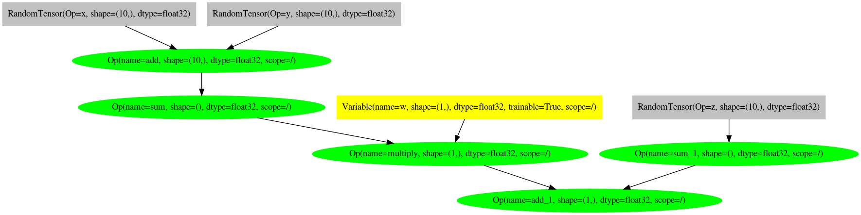
Graph visualization
Similarly to Theano, it is possible to display the computational graph of the code written as follows:
#!/usr/bin/env python
# -*- coding: utf-8 -*-

__author__ = "Randall Balestriero"

import symjax.tensor as T
import matplotlib.pyplot as plt
from symjax.viz import compute_graph

x = T.random.randn((10,), name="x")
y = T.random.randn((10,), name="y")
z = T.random.randn((10,), name="z")

w = T.Variable(T.ones(1), name="w")
out = (x + y).sum() * w + z.sum()

graph = compute_graph(out)
graph.draw("file.png", prog="dot")


import matplotlib.image as mpimg

img = mpimg.imread("file.png")
plt.figure(figsize=(15, 5))
imgplot = plt.imshow(img)
plt.xticks()
plt.yticks()
plt.tight_layout()
Clone: one line multipurpose graph replacement
In most current packages, the ability to perform an already define computation graph but with altered nodes is cumbersone. Some specific involve the use of layers as in Keras where one can feed any value hence allow to compute a feedforward pass without much changes but if one had to replace a specific variable or more complex part of a graph no tools are available. In Theano, the clone function allowed to do such thing and it implemented in SymJAX as well. As per the below example, it is clear how the clone utility allows to get an already defined computational graph and replace any subgraph in it with another based on a node->node mapping:
import numpy as np
import symjax
import symjax.tensor as T

# we create a simple mapping with 2 matrix multiplications interleaved
# with nonlinearities
x = T.Placeholder((8,), "float32")
w_1 = T.Variable(T.random.randn((16, 8)))
w_2 = T.Variable(T.random.randn((2, 16)))

# the output can be computed easily as
output = w_2.dot(T.relu(w_1.dot(x)))

# now suppose we also wanted the same mapping but with a noise input
epsilon = T.random.randn((8,))

output_noisy = output.clone({x: x + epsilon})

f = symjax.function(x, outputs=[output, output_noisy])

for i in range(10):
    print(f(np.ones(8)))

# [array([-14.496595,   8.7136  ], dtype=float32), array([-11.590391 ,   4.7543654], dtype=float32)]
# [array([-14.496595,   8.7136  ], dtype=float32), array([-30.038504,  26.758451], dtype=float32)]
# [array([-14.496595,   8.7136  ], dtype=float32), array([-19.214798,  19.600328], dtype=float32)]
# [array([-14.496595,   8.7136  ], dtype=float32), array([-12.927457,  10.457445], dtype=float32)]
# [array([-14.496595,   8.7136  ], dtype=float32), array([-19.486668,  17.367273], dtype=float32)]
# [array([-14.496595,   8.7136  ], dtype=float32), array([-31.634314,  24.837488], dtype=float32)]
# [array([-14.496595,   8.7136  ], dtype=float32), array([-19.756075,  12.330083], dtype=float32)]
# [array([-14.496595,   8.7136  ], dtype=float32), array([-38.9738  ,  31.588022], dtype=float32)]
# [array([-14.496595,   8.7136  ], dtype=float32), array([-19.561726,  12.192366], dtype=float32)]
# [array([-14.496595,   8.7136  ], dtype=float32), array([-33.110832,  30.104563], dtype=float32)]
Scopes, Operations/Variables/Placeholders naming and accessing
Accessing, naming variables, operations and placeholders. This is done in a similar way as in the vanilla Tensorflow form with scopes and EVERY of the variable/placeholder/operation is named and located with a unique identifier (name) per scope. If during creation both have same names, the original name is augmented with an underscore and interger number, here is a brief example:
import symjax
import symjax.tensor as T

# scope/graph naming and accessing

value1 = T.Variable(T.ones((1,)))
value2 = T.Variable(T.zeros((1,)))

g = symjax.Graph("special")
with g:
    value3 = T.Variable(T.zeros((1,)))
    value4 = T.Variable(T.zeros((1,)))
    result = value3 + value4

    h = symjax.Graph("inversion")
    with h:
        value5 = T.Variable(T.zeros((1,)))
        value6 = T.Variable(T.zeros((1,)))
        value7 = T.Variable(T.zeros((1,)), name="w")


print(g.variables)
# {'unnamed_variable': Variable(name=unnamed_variable, shape=(1,), dtype=float32, trainable=True, scope=/special/),
#  'unnamed_variable_1': Variable(name=unnamed_variable_1, shape=(1,), dtype=float32, trainable=True, scope=/special/)}

print(h.variables)
# {'unnamed_variable': Variable(name=unnamed_variable, shape=(1,), dtype=float32, trainable=True, scope=/special/inversion/),
# 'unnamed_variable_1': Variable(name=unnamed_variable_1, shape=(1,), dtype=float32, trainable=True, scope=/special/inversion/),
# 'w': Variable(name=w, shape=(1,), dtype=float32, trainable=True, scope=/special/inversion/)}

print(h.variable("w"))
# Variable(name=w, shape=(1,), dtype=float32, trainable=True, scope=/special/inversion/)

# now suppose that we did not hold the value for the graph g/h, we can still
# recover a variable based on the name AND the scope

print(symjax.get_variables("/special/inversion/w"))
# Variable(name=w, shape=(1,), dtype=float32, trainable=True, scope=/special/inversion/)

# now if the exact scope name is not know, it is possible to use smart indexing
# for example suppose we do not remember, then we can get all variables named
# 'w' among scopes

print(symjax.get_variables("*/w"))
# Variable(name=w, shape=(1,), dtype=float32, trainable=True, scope=/special/inversion/)

# if only part of the scope is known, all the variables of a given scope can
# be retreived

print(symjax.get_variables("/special/*"))
# [Variable(name=unnamed_variable, shape=(1,), dtype=float32, trainable=True, scope=/special/),
#  Variable(name=unnamed_variable_1, shape=(1,), dtype=float32, trainable=True, scope=/special/),
#  Variable(name=unnamed_variable, shape=(1,), dtype=float32, trainable=True, scope=/special/inversion/),
#  Variable(name=unnamed_variable_1, shape=(1,), dtype=float32, trainable=True, scope=/special/inversion/),
#  Variable(name=w, shape=(1,), dtype=float32, trainable=True, scope=/special/inversion/)]

print(symjax.get_ops("*add"))
# Op(name=add, shape=(1,), dtype=float32, scope=/special/)
Graph Saving and Loading
An important feature of SymJAX is the easiness to reset, save, load variables. This is crucial in order to save a model and being to reloaded (in a possibly different script) to keep using it. In our case, a computational graph is completely defined by its structure and the values of the persistent nodes (the variables). Hence, it is enough to save the variables. This is done in a very explicit manner using the numpy.savez utility where the saved file can be accessed from any other script, variables can be loaded, accessed, even modified, and then reloaded inside the computational graph. Here is a brief example:
import symjax
import symjax.tensor as T

g = symjax.Graph("model1")
with g:
    learning_rate = T.Variable(T.ones((1,)))
    with symjax.Graph("layer1"):
        W1 = T.Variable(T.zeros((1,)), name="W")
        b1 = T.Variable(T.zeros((1,)), name="b")
    with symjax.Graph("layer2"):
        W2 = T.Variable(T.zeros((1,)), name="W")
        b2 = T.Variable(T.zeros((1,)), name="b")

# define an irrelevant loss function involving the parameters
loss = (W1 + b1 + W2 + b2) * learning_rate

# and a train/update function
train = symjax.function(
    outputs=loss, updates={W1: W1 + 1, b1: b1 + 2, W2: W2 + 2, b2: b2 + 3}
)

# pretend we train for a while
for i in range(4):
    print(train())

# [0.]
# [8.]
# [16.]
# [24.]

# now say we wanted to reset the variables and retrain, we can do
# either with g, as it contains all the variables
g.reset()
# or we can do
symjax.reset_variables("*")
# or if we wanted to only reset say variables from layer2
symjax.reset_variables("*layer2*")

# now that all has been reset, let's retrain for a while
# pretend we train for a while
for i in range(2):
    print(train())

# [0.]
# [8.]

# now resetting is nice, but we might want to save the model parameters, to
# keep training later or do some other analyses. We can do so as follows:
g.save_variables("model1_saved")
# this would save all variables as they are contained in g. Now say we want to
# only save the second layer variables, if we had saved the graph variables as
# say h we could just do ``h.save('layer1_saved')''
# but while we do not have it, we recall the scope of it, we can thus do
symjax.save_variables("*layer1*", "layer1_saved")
# and for the entire set of variables just do
symjax.save_variables("*", "model1_saved")

# now suppose that after training or after resetting
symjax.reset_variables("*")

# one wants to recover the saved weights, one can do
symjax.load_variables("*", "model1_saved")
# in that case all variables will be reloaded as they were in model1_saved,
# if we used symjax.load('*', 'layer1_saved'), an error would occur as not all
# variables are present in this file, one should instead do
# (in this case, this is redundant as we loaded everything up above)
symjax.load_variables("*layer1*", "layer1_saved")

# we can now pretend to keep training our model form its saved state
for i in range(2):
    print(train())

# [16.]
# [24.]
Wrap: Jax function/computation to SymJAX Op
The computation in Jax is done eagerly similarly to TF2 and PyTorch. In SymJAX the computational graph definition is done a priori with symbolic variables. That is, no actual computations are done during the graph definition, once done the graph is compiled with proper inputs/outputs/updates to provide the user with a compiled function executing the graph. This graph thus involves various operations, one can define its own in the two following way. First by combining the already existing SymJAX function, the other by creating it in pure Jax and then wrapping it into a SymJAX symbolic operation as demonstrated below.
#!/usr/bin/env python
# -*- coding: utf-8 -*-

import symjax as sj
import jax.numpy as jnp

__author__ = "Randall Balestriero"

# suppose we want to compute the mean-squared error between two vectors
x = sj.tensor.random.normal((10,))
y = sj.tensor.zeros((10,))

# one way is to do so by combining SymJAX functions as
mse = ((x - y) ** 2).sum()
# notice that the basic operators are overloaded and implicitly call SymJAX ops

# another solution is to create a new SymJAX Op from a jax computation as
# follows


def mse_jax(x, y):
    return jnp.sum((x - y) ** 2)


# wrap the jax computation into a SymJAX Op that can then be used as any
# SymJAX function
mse_op = sj.tensor.jax_wrap(mse_jax)
also_mse = mse_op(x, y)
print(also_mse)
# Tensor(Op=mse_jax, shape=(), dtype=float32)


# ensure that both are equivalent
f = sj.function(outputs=[mse, also_mse])
print(f())
# [array(6.0395503, dtype=float32), array(6.0395503, dtype=float32)]
A SymJAX computation graph can not be partially defined with Jax computation, the above thus provides an easy way to wrap Jax computations into a SymJAX Op which can then be put into the graph as any other SymJAX provided Ops.
Wrap: Jax class to SymJAX class
One might have defined a Jax class, with a constructor possibly taking some constant values and some jax arrays, performing some computations, setting some attributes, and then interacting with those attributes when calling the class methods. It would be particularly easy to pair such already implemented classes with SymJAX computation graph. This can be done as follows:
#!/usr/bin/env python
# -*- coding: utf-8 -*-

import symjax as sj
import symjax.tensor as T
import jax.numpy as jnp

__author__ = "Randall Balestriero"


class product:
    def __init__(self, W, V=1):
        self.W = jnp.square(V * W * (W > 0).astype("float32"))
        self.ndim = self.compute_ndim()

    def feed(self, x):
        return jnp.dot(self.W, x)

    def compute_ndim(self):
        return self.W.shape[0] * self.W.shape[1]


wrapped = T.wrap_class(product, method_exceptions=["compute_ndim"])


a = wrapped(T.zeros((10, 10)), V=T.ones((10, 10)))
x = T.random.randn((10, 100))

print(a.W)
# (Tensor: name=function[0], shape=(10, 10), dtype=float32)

print(a.feed(x))
# Op(name=feed, shape=(10, 100), dtype=float32, scope=/)

f = sj.function(outputs=a.feed(x))

f()
As can be seen, there is some restrictions. First, the behavior inside the constructor of the original class should be fixed as it will be executed once by the wrapper in order to map the constructor computations into SymJAX. Second, any jax array update done internally will break the conversion as such operations are only allowed for Variables in SymJAX, hence some care is needed. More flexibility will be provided in future versions.
Amortized Variational Inference
We briefly describe some key components of SymJAX.
The principles of AVI
Reinforcement Learning
We briefly describe some key components of SymJAX.
Notations
immediate reward \(r_t\) is observed from the environment at state \(𝑠_{t}\) by performing action \(𝑎_{t}\)
total discounted reward \(𝐺_t(γ)\) often abbreviated as \(𝐺_t\) and defined as
\[𝐺_t = Σ_{t'=t+1}^{T}γ^{t'-t-1}r_t\]action-value function \(Q_{π}(𝑠,𝑎)\) is the expected return starting from state 𝑠, following policy 𝜋 and taking action 𝑎
\[Q_{π}(𝑠,𝑎)=E_{π}[𝐺_{t}|𝑠_{t} = 𝑠,𝑎_{t}=𝑎]\]state-value function \(V_{π}(𝑠)\) is the expected return starting from state 𝑠 following policy 𝜋 as in
\[\begin{split}V_{π}(𝑠)&=E_{π}[𝐺_{t}|𝑠_{t} = 𝑠]\\ &=Σ_{𝑎 ∈ 𝐴}π(𝑎|𝑠)Q_{π}(𝑠,𝑎)\end{split}\]in a deterministic policy setting, one has directly \(V_{π}(𝑠)=Q_{π}(𝑠,π(𝑠))\). in a greedy policy one might have \(V^{*}_{π}(𝑠)=\max_{𝑎∈𝐴}Q_{π}(𝑠,𝑎)\) where \(V^{*}_{π}\) is the best value of a state if you could follow an (unknown) optimum policy.
TD-error
- \(𝛿_t=r_t+γQ(𝑠_{t+1},𝑎_{t+1})-Q(𝑠_{t},𝑎_{t})\)
advantage value : how much better it is to take a specific action compared to the average at the given state
\[\begin{split}A(s_t,𝑎_t)&=Q(𝑠_t,𝑎_t)-V(𝑠_t)\\ A(𝑠_t,𝑎_t)&=E[r_{t+1}+ γ V(𝑠_{t+1})]-V(𝑠_t)\\ A(𝑠_t,𝑎_t)&=r_{t+1}+ γ V(𝑠_{t+1})-V(𝑠_t)\end{split}\]The formulation of policy gradients with advantage functions is extremely common, and there are many different ways of estimating the advantage function used by different algorithms.
probability of a trajectory \(τ=(s_0,a_0,...,s_{T+1})\) is given by
\[p(τ|θ)=p_{0}(s_0)Π_{t=0}^{T}p(𝑠_{t+1}|𝑠_{t},𝑎_{t})π_{0}(𝑎_{t}|𝑠_{t})\]
Policy gradient and REINFORCE
Policy gradient and REINFORCE : Policy gradient methods are ubiquitous in model free reinforcement learning algorithms — they appear frequently in reinforcement learning algorithms, especially so in recent publications. The policy gradient method is also the “actor” part of Actor-Critic methods. Its implementation (REINFORCE) is also known as Monte Carlo Policy Gradients. Policy gradient methods update the probability distribution of actions \(π(a|s)\) so that actions with higher expected reward have a higher probability value for an observed state.
- needs to reach end of episode to compute discounted rewards and train the model
- only needs an actor (a.k.a policy) network
- noisy gradients and high variance => instability and slow convergence
- fails for trajectories having a cumulative reward of 0
Tricks
- normalizing discounter rewards (or advantages) : In practice it can can also be important to normalize these. For example, suppose we compute [discounted cumulative reward] for all of the 20,000 actions in the batch of 100 Pong game rollouts above. One good idea is to “standardize” these returns (e.g. subtract mean, divide by standard deviation) before we plug them into backprop. This way we’re always encouraging and discouraging roughly half of the performed actions. Mathematically you can also interpret these tricks as a way of controlling the variance of the policy gradient estimator.